3 Allocation
Once we’ve decided how many participants we need in our trial, we need to determine how they will each be assigned to a trial arm. This is process is known as allocation (or sometimes as randomization). Before we think about methods for allocation, we are going to spend some time talking about bias.
3.1 Bias
In statistics, bias is a systematic tendency for the results of our analysis to be different from the true value. We see this particularly when we are using sample data to estimate a parameter. We will revisit what we have learned in previous courses about bias before going on to see how it affects RCTs.
Definition 3.1 (Bias of an estimate) Suppose that \(T\) is a statistic calculated to estimate a parameter \(\theta\). The bias of \(T\) is \[E\left(T\right) - \theta.\] If the bias of \(T\) is zero, we say that \(T\) is an unbiased estimator of \(\theta\).
An example you will have seen before is the standard deviation. If we have some data \(x_1,\,\ldots,x_n\) that are IID \(N\left(\mu,\,\sigma^2\right)\), we can calculate the sample variance
\[ s^2 = \frac{1}{n}\sum\limits_{i=1}^n\left(x_i - \bar{x}\right)^2 .\]
In this case, \(E\left(s^2\right) \neq {\sigma^2}\) (you’ve probably seen this proved so we’re not going to prove it now), and \(s^2\) is a biased estimator of \(\sigma^2\). However, we know that
\[E \left(\frac{n}{n-1}s^2\right) = \sigma^2,\] and therefore we can apply this correction to the sample variance \(s^2\) to produce an unbiased estimate of the population variance \(\sigma^2\). Here, the sample are representative of the population, but the size of the sample leads to some bias.
Now, suppose our sample \(x_1,\ldots,x_n\) were drawn from \(N\left(\mu,\sigma^2\right)\), but were not independent of one another. Then, neither our estimator \(s^2\), nor our bias-corrected estimator \(\frac{n}{n-1}s^2\) would have expected value \(\sigma^2\). Furthermore, we cannot use our sample \(x_1,\ldots,x_n\) to produce an unbiased estimator of \(\sigma^2\), or even of the mean \(\mu\).
This scenario is much closer to what we mean when we talk about bias in a clinical trial setting. Suppose we are testing some new treatment \(T\) against the standard \(C\). We measure some outcome \(X\) for each patient, and our hypothesis is that \(X\) behaves differently for those in the treatment group than for those in the control group. It is common practice to express this additively, \[E\left(X\right) = \mu + \tau,\] where \(\tau\) is our treatment effect, which we can estimate using the difference in the groups’ means, \(\bar{X}_T - \bar{X}_C\). Our null hypothesis is that \(\tau = 0\), and our alternative hypothesis is that \(\tau\neq{0}\), and therefore an estimate of \(\tau\) from our data is very important! Put equivalently, it is important that there is no bias in our estimates of \(\bar{X}_C\) and \(\bar{X}_T\).
Usually, what this comes down to is that the assumption that the data are independent, identically distributed random variables from the relevant distributions (which we have already relied on a lot for our sample size calculations) has been violated in some way.
Example 3.1 Historically, women and the elderly are underrepresented in clinical trials (Cottingham and Fisher (2022)) and results are often translated from young or middle aged healthy men to these other groups (Vitale et al. (2017)). This isn’t reasonable, since women have very different hormonal activity from men, causing them to often react differently to drugs compared to men involved in the trial. The standard dose (based on trials with mostly male participants) can also be too high for many women. The complicated nature of women’s hormones is sometimes even given as a reason for not including them in the trial. Women and elderly people are also both more likely to have adverse effects to drugs in some fields.
There are also ethical reasons behind the low numbers of women in trials, especially phase I and phase II trials. If a woman is possibly pregnant (and trials tend to be extremely cautious in deciding who might be pregnant!) then they are quite often excluded, in order to protect the (actual or hypothetical) fetus. Indeed, in 1977 the Food and Drug Administration (FDA) in the US recommended that women be excluded from phase I and II trials (Health (2023)) as a result of some severe cases of fetuses being harmed by drugs (especially Thalidamide) . This means that even some very mainstream drugs, for example antihistamines (Kar et al. (2012)), haven’t been tested for safety/efficacy during pregnancy, as well as some (for example HIV treatments) that would be of huge benefit to many many pregnant women. This article is an interesting read if you would like to know more.
In the above example, the trial cohort is very deliberately (and arguably sometimes defensibly) not representative of the target population. However, bias can creep into trials in a number of ways.
3.1.1 Where does bias come from?
Having established that bias is a serious issue in clinical trials, we will think about several sources of bias. Some of these we will elaborate on as we get to the relevant part of methodology. Most sources of bias creep in during the allocation or selection phase.
Selection bias
Selection bias occurs when certain patients or subjects are systematically more (or less) likely be entered into the trial because of the treatment they will receive. In a properly run trial this isn’t possible, because it is only after a participant has been recruited that their treatment is chosen. If a medical professional is not comfortable with a particular patient potentially receiving one of the possible treatments, then that patient should not be entered into the trial at all. If there are many such [technically eligible] patients, then this might cause the estimated treatment effect to be worryingly far from the true population treatment effect, since the recruited group of participants would not be very representative of the true population (this is not technically selection bias, but it comes from the same problem).
It may happen that the doctor knows which treatment a patient would be given, for example if the allocation follows some deterministic pattern, or is fully known to the doctor in advance. Consciously or subconsciously this knowledge may influence the description they give to potential participants, and this in turn may affect which patients sign up, and the balance of the groups. In practice there should be various safeguards against this situation.
Allocation bias
Mathematically, allocation bias is similar to selection bias, but instead of coming from human ‘error’, it arises from the random process of allocation.
Suppose a trial investigates a drug that turns out to have a much stronger effect on male patients than on female patients. The cohort of recruited participants are randomised into treatment and control groups, and it happens that there is a much smaller proportion of female patients in one group than the other. This will distort the estimated treatment effect.
We will investigate various strategies for randomization designed to address this issue for known factors.
Example 3.2 This example is framed in terms of selection bias, but applies equally to allocation bias
Suppose we run a trial comparing a surgical (S) and a non-surgical (N) treatment for some condition. Patients who are eligible are given the opportunity to join the trial by a single doctor.
The severity of the disease is graded as 1 (less serious) or 2 (more serious) for each patient. Across the full group of patients, proportion \(\lambda\) have severity 1 and proportion \(1-\lambda\) have severity 2.
Our primary outcome is survival time, \(X\), which depends on the severity of disease:
\[\begin{align*} E\left(X\mid{1}\right) & = \mu_1\\ E\left(X\mid{2}\right) & = \mu_2 \end{align*}\]
and we assume \(\mu_1>\mu_2\).
For the overall trial group, for untreated patients we have
\[ E\left(X\right) = \mu = \lambda \mu_1 + \left(1-\lambda\right)\mu_2.\] Suppose that for treatment group \(N\), the expected survival time increase by \(\tau_N\), and similarly for group \(S\), so that we have
\[\begin{align*} E\left(X\mid{N,1}\right) & = \mu_1 + \tau_N\\ E\left(X\mid{N,2}\right) & = \mu_2 + \tau_N\\ E\left(X\mid{S,1}\right) & = \mu_1 + \tau_S\\ E\left(X\mid{S,2}\right) & = \mu_2 + \tau_S. \end{align*}\]
If all patients were admitted with equal probability to the trial (ie. independent of the severity of their disease) then the expected survival time for group \(N\), \(E\left(X\mid{N}\right)\), would be
\[\begin{align*} E\left(X\mid{1,N}\right)P\left(1\mid{N}\right) + E\left(X\mid{2,N}\right)P\left(2\mid{N}\right)& = \left(\mu_1 + \tau_N\right)\lambda + \left(\mu_2+\tau_N\right)\left(1-\lambda\right)\\ & = \mu + \tau_N. \end{align*}\]
Similarly, the expected survival time in group \(S\) would be \(\mu+\tau_S\), and the treatment effect difference between the two would be \(\tau = \tau_N - \tau_S\) and the trial is unbiased.
Suppose that although all eligible patients are willing to enter the trial, the doctor is reticent to subject patients with more severe disease (severity 2) to the surgical procedure. This is reflected in the way they explain the trial to each patient, particularly those with severity 2 whom the doctor knows will be assigned to group \(S\). In turn this leads to a reduced proportion \(q = 1-p\) of those with severity 2 assigned to surgery entering the trial (event \(A\)):
\[\begin{align*} P\left(A\mid{N,1}\right) = P\left(A\mid{S,1}\right) = P\left(A\mid{N,2}\right) & = 1 \\ P\left(A\mid{S,2}\right) & = 1-p = q. \end{align*}\]
Since our analysis is based only on those who enter the trial, our estimated treatment effect will be
\[E\left(X\mid{A, N}\right) - E\left(X\mid{A, S}\right). \] We can split these according to disease severity, so that
\[E\left(X\mid{A,N}\right) = E\left(X\mid{A,N,1}\right)P\left(1\mid{A,N}\right) + E\left(X\mid{A,N,2}\right)P\left(2\mid{A,N}\right) \] and similarly for group \(S\).
We can calculate \(P\left(1\mid{A,N}\right)\) using Bayes’ theorem,
\[\begin{align*} P\left(1\mid{A,N}\right) & = \frac{P\left(A\mid{1,N}\right)P\left(1\mid{N}\right)}{P\left(A\mid{N}\right)}\\ & = \frac{P\left(A\mid{1,N}\right)P\left(1\mid{N}\right)}{P\left(A\mid{N,1}\right)P\left(1\mid{N}\right) + P\left(A\mid{N,2}\right)P\left(2\mid{N}\right)} \\ &= \frac{1\times{\lambda}}{1\times {\lambda} + 1 \times{\left(1-\lambda\right)}}\\ & = \lambda. \end{align*}\] Therefore we also have \(P\left(2\mid{A,N}\right) = 1 -P\left(1\mid{A,N}\right) = 1-\lambda\).
Following the same process for group \(S\), we arrive at
\[\begin{align*} P\left(1\mid{A,S}\right) & = \frac{P\left(A\mid{1,S}\right)P\left(1\mid{S}\right)}{P\left(A\mid{S}\right)}\\ & = \frac{P\left(A\mid{1,S}\right)P\left(1\mid{S}\right)}{P\left(A\mid{S,1}\right)P\left(1\mid{S}\right) + P\left(A\mid{S,2}\right)P\left(2\mid{S}\right)} \\ & = \frac{\lambda}{\lambda + q\left(1-\lambda\right)}, \end{align*}\]
which we will call \(b\).
Notice that \(P\left(2\mid{S}\right)= 1-\lambda\), since it is not conditional on actually participating in the trial. Therefore,
\[\begin{align*} E\left(X\mid{A,N}\right) & = E \left(X\mid{N,1}\right)P\left(1\mid{A,N}\right) + E \left(X\mid{N,2}\right)P\left(2\mid{A,N}\right) \\ & = \left(\mu_1 + \tau_N\right)\lambda + \left(\mu_2 + \tau_N\right)\left(1-\lambda\right) \\ & = \lambda\mu_1 + \left(1-\lambda\right)\mu_2 + \tau_N \end{align*}\]
and
\[\begin{align*} E\left(X\mid{A,S}\right) & = E \left(X\mid{S,1}\right)P\left(1\mid{A,S}\right) + E \left(X\mid{S,2}\right)P\left(2\mid{A,S}\right) \\ & = \left(\mu_1 + \tau_S\right)b + \left(\mu_2 + \tau_S\right)\left(1-b\right) \\ & = b\mu_1 + \left(1-b\right)\mu_2 + \tau_S. \end{align*}\]
From here, we can calculate the expected value of the estimated treatment effect \(\hat\tau\) as (substituting our equation for \(b\) and rearranging):
\[\begin{align*} E\left(X\mid{A,N}\right) - E\left(X\mid{A,S}\right) & = \tau_N - \tau_S + \left(\lambda - b\right)\left(\mu_1 - \mu_2\right) \\ & = \tau_N - \tau_S - \frac{p\lambda\left(1-\lambda\right)\left(\mu_1 - \mu_2\right)}{\lambda + q\left(1-\lambda\right)}, \end{align*}\]
where the third term represents the bias.
Notice that if \(q=1-p = 1\), then there is no bias. There is also no bias if \(\mu_1 = \mu_2\), ie. if there is no difference between the disease severity groups in terms of survival time.
Assuming \(\mu_1 - \mu_2 >0\), then the bias term is positive and
\[E\left(\hat\tau\right) = E\left(X\mid{A,N}\right)- E\left(X\mid{A,S}\right) < \tau_N - \tau_S.\] If \(N\) is the better treatment, then \(\tau_N - \tau_S>0\) and the bias will cause the trial to underplay the treatment effect. Conversely, if \(S\) is better, then \(\tau_N-\tau_S<0\) and the trial will exaggerate the treatment effect. Essentially, this is because more severely ill patients have been assigned to \(N\) than to \(S\), which reduces the average survival time for those in group \(N\).
Assessment bias
Measurements are made on participants throughout the trial. These measurements will often be objective, for example the patients’ weight, or concentration of blood sugar. However, some types of measurement are much more subject to the individual practitioner assessing the patient. For example, many skin conditions are assessed visually, for example estimating the proportion of the body affected. Measuring quantities such as quality of life or psychological well-being involve many subjective judgements on the part of both patient and clinician.
Clearly it is ideal for both the patient and the clinician not to know which arm of the trial the patient was part of (this is known as a double blind trial). For treatments involving drugs, this is usually straightforward. However, for surgical interventions it is often impossible to keep a trial ‘blind’, and for interventions involving therapy (for example cognitive behavioural therapy) it is impossible for the patient to be unaware. In this situation, it is possible for the patient or clinician’s judgement to be affected by their knowledge of the allocation, thus affecting the estimated treatment effect.
Slight aside: publication bias
In most areas of science, including clinical trials, the ultimate aim is to affect practice. This is usually done by publishing a write-up of the trial, including its design, methods, analysis and results, and publishing that in a [medical] journal. These are peer-reviewed, which means that experts from the relevant field are asked to review submitted papers, and either reject or accept them (usually conditional on some revision). These reviewers advise the editor of the journal, who ultimately decides whether or not the paper will be published.
There is compelling evidence that papers reporting positive / conclusive results are more likely to be published than papers about [viable] trials that ultimately fail to reject the null hypothesis. As we know, in most cases if the null hypothesis is rejected this is indicative that there is a true treatment difference. However, sometimes by random chance a trial will detect a difference even when there isn’t one (approximately 5% of the time if \(\alpha=0.05\)). If these papers are disproportionately likely to be published, the body of literature will not reflect the truth, and there may be serious implications for practice. This is a huge issue in the pharmaceutical industry, and one from which we can’t escape. If you’d like to learn more about it the book ‘Bad Pharma’ by Goldacre (2012) is an excellent source.
Measures are being taken to prevent this: for example, leading medical journal The Lancet insists that any clinical trial related paper is registered with them before the first participant has been recruited, with details of the design and statistical analysis plan. This is then reviewed before the trial begins.
3.1.2 Implications for allocation
Historically (and probably still, to an extent), clinical trials have not necessarily used random allocation to assign participants to groups. Altman and Bland (1999) gives an overview of why this has led to bias, and gives some examples.
Sometimes analyses compare groups in serial, so that \(N_A\) patients one year (say) form the control group, and \(N_B\) patients in a subsequent year, who are given treatment \(B\), form the intervention group. In this scenario it is impossible to control for all other changes that have occurred with time, and this leads to a systematic bias, usually in favour of treatment \(B\).
Given the need for contemporary control participants, the question becomes how to assign participants to each group. If the clinician is able to choose who receives which treatment, or if each patient is allowed to choose or refuse certain treatments, this is almost certain to introduce bias. This is avoided by using random allocation.
There are two important aspects to the allocation being random that we will draw attention to.
- Every patient should have the same probability of being assigned to each treatment group.
- The treatment group for a particular patient should not be able to be predicted.
Point 1 is important because, as we have already mentioned, the statistical theory we use to plan and analyse the trial is based on the groups being random samples from the population.
Point 2 is important to avoid biases that come through the assignment of a particular patient being known either in advance or after the fact. There are some approaches that ‘pass’ the first point, but fail at the second. As well as strict alternation (\(ABABAB\ldots\)), some such methods use patient characteristics such as date of birth or first letter of surname, which is not related to the trial outcome, but which enables allocations to be predicted.
We will now explore some commonly used methods of allocation. We will usually assume two equally sized groups, \(A\) and \(B\), but it is simple to generalize to three or more groups, or to unequal allocation.
3.2 Allocation methods
In this chapter, and in the computer practical on allocation, we will study the behaviour of various allocation methods by implementing them many times. This gives us an idea of how variable the results are, especially in terms of being likely to introduce bias or reduce power. In almost all real trials, patients are allocated and begin treatment as they arrive, and this may happen over the course of weeks or months. The allocation that is generated is the final allocation. It is therefore important to minimise the probability of it being a poor one!
3.2.1 Simple random allocation
Perhaps intuitively the most simple method is a ‘toin coss’, where each participant has a probability 0.5 of being placed in each group. As participants arrive, assignment \(C\) or \(T\) is generated (with equal probability). Statistically, this scheme is ideal, since it generates the random sample we need, and the assignment of each participant is statistically independent of that of all other participants. It also doesn’t require a ‘master’ randomisation; several clinicians can individually assign participants to treatment groups in parallel and the statistical properties are maintained.
This method is used effectively in many large trials, but for small trials it can be statistically problematic. The main reason for this is chance imbalance of group sizes.
Suppose we have two groups, \(T\) of size \(N_T\) and \(C\) of size \(N_C\), with \(N_T + N_C = 2n\). Patients are allocated independently with equal probability, which means
\[N_C \sim \operatorname{Bi}\left(2n,\frac{1}{2}\right), \] and similar for \(N_T\). If the two groups are of unequal size, the larger will be of some size \(N_{max}\) between \(n\) and \(2n\), such that for \(r = n+1,\,\ldots,\,2n,\)
\[\begin{align*} P\left(N_{max} = r\right) & = P\left(N_C = r\right) + P\left(N_T = r\right) \\ & = 2\binom{2n}{r}\left(\frac{1}{2}\right)^{2n}. \end{align*}\] The probability that \(N_C = N_T = n\) is
\[ P\left(N_T = N_C = n\right)= \binom{2n}{n}\left(\frac{1}{2}\right)^{2n}. \] These probabilities are shown in Figure 3.1. We can see that this method leads to very unequal groups relatively easily; with \(n=15\), \(P\left(N_{max}\geq 20\right) = 0.099\), so there is around a one in ten chance that one group will be double or more the size of the other.
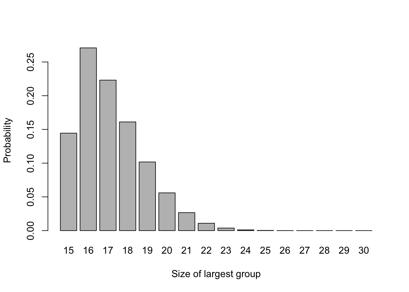
Figure 3.1: The probability distribution of largest group size for n=15.
As we have seen when thinking about sample sizes in Section 2.4, this will reduce the power \(\Psi\) of the trial, since it depends on \(\lambda\left(N_C,\,N_T\right) = \sqrt{\frac{1}{N_C} + \frac{1}{N_T}}\).
For larger trials, this imbalance will be less pronounced, for example Figure 3.2 shows the same for \(n=200\).
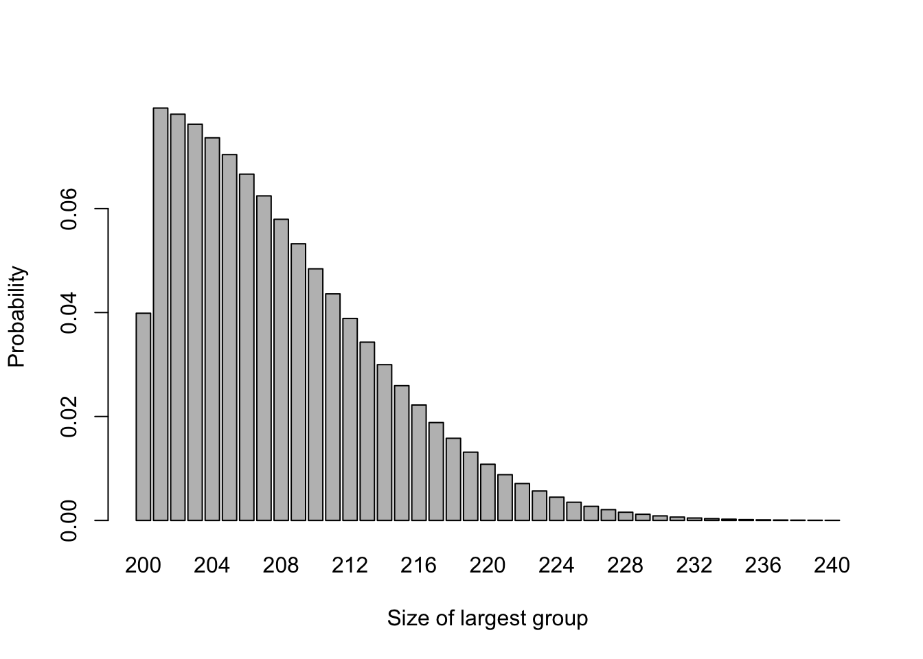
Figure 3.2: The probability distribution of largest group size for n=200.
In this case \(P\left(N_{max} \geq 220\right)=0.051\), so the chance of highly imbalanced groups is much lower. However, we may want to achieve balance on some factor thought to be important, for example sex, age group or disease state, and in this case there may be small numbers even in a large trial.
We saw in the sample size section that the greatest power is achieved when group sizes are equal, since this minimises the function
\[\lambda\left(n,m\right) = \sqrt{\frac{1}{n}+\frac{1}{m}}.\] However, with simple random sampling we can’t guarantee equal group sizes.
Example 3.3 Suppose we are designing a trial to have \(\alpha=0.05\), and our minimum detectable effect size is such that \(\frac{\tau_M}{\sigma}=1\). If 30 participants are recruited, then we can calculate the power of the study using methods from Chapter 2:
\[1-\beta = \Phi\left(\sqrt{\frac{n_T\,n_C}{30}} - 1.96\right). \] The first term in the standard normal CDF comes from the fact that
\[\left[\lambda\left(n,m\right)\right]^{-1} = \sqrt{\frac{nm}{n+m}} .\] If we have equal group sizes \(n_T=n_C=15\), then the power achieved is 78%. If the group sizes are 10 and 20, we have a power of 73%. If the group sizes are 6 and 24, the power goes down to 59%.
So, as we saw when looking at power, we don’t lose too much if the group sizes are 2:1, but a more pronounced imbalace has resulted in a much more noticeable loss. There may be other disadvantages to having such imbalance, for example increased costs, or a reduction in the amount of information gained about side effects. If this imbalance can be avoided, it should be.
3.2.2 Random permuted blocks
One commonly used method to randomly allocate participants while avoiding imbalance is to use random permuted blocks (RPBs). With RPBs we randomly generate the allocation in blocks of some predetermined size. If the blocks have size \(2m\), and there are two groups then there are \[\binom{2m}{m},\] but this method can be adapted to more than two groups and to unequal group size.
Example 3.4 If we have two groups, \(A\) and \(B\), then there are six blocks of length 4 containing two \(A\)s and two \(B\)s
\[ \begin{aligned} 1.& AABB\\ 2.& ABAB\\ 3.& ABBA\\ 4.& BAAB\\ 5.& BABA\\ 6.& BBAA. \end{aligned} \]
We can also randomly generate a sequence of numbers from \(\left\lbrace 1, 2, 3, 4, 5, 6 \right\rbrace\), where each number has equal probability. This sequence will correspond to a sequence in \(A\) and \(B\) with four times the length. In this method, each patient is equally likely to receive \(A\) and \(B\), but there will never be a difference of more than two between the size of the two groups.
For example, suppose the sequence begins \(2,1,3,6,\ldots\). Replacing each number by its block, we have \(ABAB\;AABB\;ABBA\;BBAA\;\ldots\).
One serious disadvantage of this method is that if the block size is fixed, and the doctors involved in the trial know which participants have received which treatments (which is unavoidable in cases such as surgery), then the allocation for some patients can be perfectly predicted. For blocks of size four this is true for the fourth in every block, and for the third and fourth if the first two were the same. This means that selection bias may be a problem in more than 25% of participants, which is deemed unacceptable; indeed, it fails our second point about randomization.
3.2.2.1 RPBs with random block length
The issue above can be circumvented by not only randomly choosing from a selection of blocks, but also randomly choosing the length of the block. For example, there are \[ \binom{6}{3} = 20\] possible blocks of size 6. Instead of always selecting from the six possible 4-blocks, a sampling scheme can be as follows.
- A random number \(X\) is drawn from \(\left\lbrace 4,6\right\rbrace\) to select the block length.
- A second random number \(Y\) is drawn from 1 to 6 (if the block length is four) or 1 to 20 (if the block length is 6).
- The block corresponding to \(Y\) is chosen and participants assigned accordingly.
- If more participants are needed, go back to step 1.
As well as ensuring that patients are equally likely to receive treatments \(A\) and \(B\), and that \(N_A\) and \(N_B\) can never differ by more than three, this method hugely reduces the possibility of enabling selection bias. The assignment of a patient can only be perfectly predicted if the difference is three, and this happens only for two of the twenty blocks of length six.
3.2.3 Biased coin designs and urn schemes
It may be that we prefer a method that achieves balance while retaining the pure stochasticity of simple random sampling. An advantage of RPBs was that once the sequence was generated, no computing power was needed. However, it is safe now to assume that any hospital pharmacy, nurse’s station, GP office or other medical facility will have a computer with access to the internet (or some internal database), and therefore more sophisticated methods are available. It is also very likely that all trial data may be stored on some central database, and so methods that rely on knowing the allocation so far (albeit in some encrypted form) should be possible even if there are multiple clinicians and sites involved.
Biased coin designs and urn schemes both work by adjusting the probabilities of allocation according to the balance of the design so far, such that a participant is less likely to be assigned to an over-represented group.
3.2.3.1 Biased coin designs
The biased coin design was introduced by Efron (1971), with the aim of ensuring balance whilst not becoming vulnerable to various forms of experimental bias. Efron (1971) suggested the biased coin design be used to achieve balance in terms of patient characteristics (eg. age group, sex, disease state etc.), but in this section we will think about the whole cohort (the maths for a subgroup would be the same).
Suppose we are using a biased coin design for a trial to compare two treatments, \(T\) and \(C\). At the point where some number \(n\) (not the total trial cohort) have been allocated, we can use the notation \(N_T\left(n\right)\) for the number of participants allocated to treatment \(T\), and \(N_C\left(n\right)\) for the number of participants allocated to treatment \(C\). Using these, we can denote the imbalance in treatment numbers by
\[ D\left(n\right) = N_T\left(n\right) - N_C\left(n\right).\] We use the imbalance \(D\left(n\right)\) to alter the probability of allocation to each treatment in order to restore (or maintain) balance in the following way:
- If \(D\left(n\right)=0\), allocate patient \(n+1\) to treatment \(T\) with probability \(\frac{1}{2}\).
- If \(D\left(n\right)>0\), allocate patient \(n+1\) to treatment \(T\) with probability \(P\).
- If \(D\left(n\right)<0\), allocate patient \(n+1\) to treatment \(T\) with probability \(1-P\).
where \(P\in\left(\frac{1}{2}, 1\right)\).
Question: What would happen if \(P=\frac{1}{2}\) or \(P=1\)?
If, at some point in the trial, we have \(\lvert D\left(n\right)\rvert = j\), for some \(j>0\), then we must have either
\[ \lvert D\left(n+1\right)\rvert = j+1 \] or \[ \lvert D\left(n+1\right)\rvert = j-1 .\] Because of the way we have set up the scheme,
\[ p\big(\lvert D\left(n+1\right)\rvert = j+1\big) = 1-P \] and
\[ p\big(\lvert D\left(n+1\right)\rvert = j-1\big) = P.\] If \(\lvert D\left(n\right) \rvert = 0\), ie. the scheme is in exact balance after \(n\) allocations, then we must have \(\lvert D\left(n+1\right)\rvert = 1\).
The absolute imbalances therefore form a simple random walk on the non-negative integers, with transition probabilities
\[ \begin{aligned} P\bigg(\lvert D\left(n+1\right) \rvert = 1 \; \bigg| \;\lvert D\left(n\right)\rvert=0\bigg)& = 1\\ P\bigg(\lvert D\left(n+1\right) \rvert = j+ 1 \; \bigg| \; \lvert D\left(n\right)\rvert=j\bigg)& = 1 - P\\ P\bigg(\lvert D\left(n+1\right) \rvert = j-1 \; \bigg| \; \lvert D\left(n\right)\rvert=j\bigg)& = P \end{aligned} \] Figure 3.3 shows four realisations of this random walk with \(P=0.667\) (Efron’s preferred value). We see that sometimes the imbalance gets quite high, but in general it isn’t too far from 0.
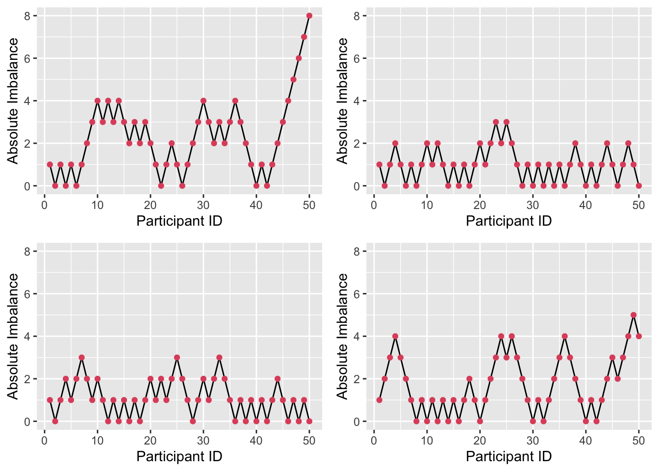
Figure 3.3: Absolute imbalance for a biased-coin scheme with \(P=0.667\).
Figure 3.4 shows four realisations of the random walk with \(P=0.55\). Here, the imbalance is able to get very high (note the change in \(y\)-axis); for example in the first plot, if we stopped the trial at \(n=50\) we would have 34 participants in one arm and only 16 in the other.
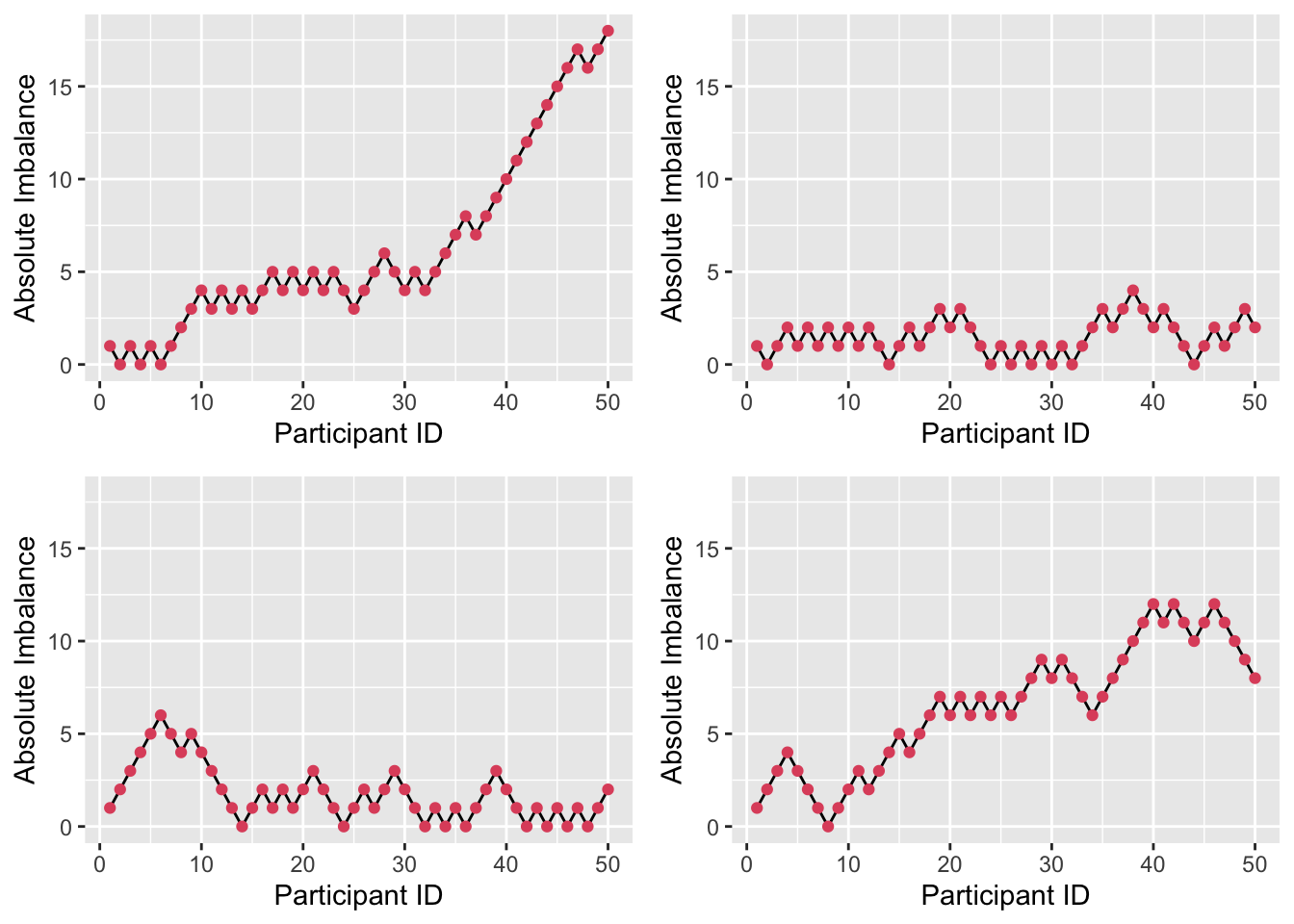
Figure 3.4: Absolute imbalance for a biased-coin scheme with \(P = 0.55\).
By contrast, with \(P=0.9\) as in Figure 3.5, there is much less imbalance. However, this brings with it greater predictability. Although allocation is always random, given some degree of imbalance (likely to be known about by those executing the trial), the probability of guessing the next allocation correctly is high (0.9). This invites the biases we have been trying to avoid, albeit in an imperfect form.
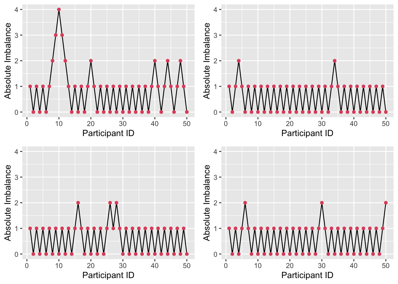
Figure 3.5: Absolute imbalance for a biased-coin scheme with \(P = 0.9\).
Efron’s suggestion for implementation was that each clinician would received an unordered stack of envelopes. Each would contain three more envelopes, each with instructions covering one of the three possible cases (\(\lvert D\left(n\right)\rvert<0,\,\lvert D\left(n\right)\rvert=0\) and \(\lvert D\left(n\right)\rvert>0\)). The clinician would open the appropriate envelope and implement the instruction. Remember this was 1971!
A big disadvantage to the biased coin scheme is that the same probability is used regardless of the size of the imbalance (assuming it isn’t zero). In the next section, we introduce a method where the probability of allocating the next patient to the underrepresented treatment gets larger as the imbalance grows.
3.2.3.2 Urn models
Urn models for treatment allocation use urns in the way that you might well remember from school probability (or indeed often we had drawers of socks). They were first applied to clinical trials by Wei (1978). In this setting, the urn starts off with a ball for each treatment, and a ball is added to the urn each time a participant is allocated. The ball is labelled according to the treatment allocation that participant did not receive.
To allocate the next participant, a ball is drawn from the urn. If the allocations at this point are balanced, then the participant has equal probability of being allocated to each treatment. If there is imbalance, there will be more balls labelled by the underrepresented treatment, and so the participant is more likely to be allocated to that one. The greater the imbalance, the higher the probability of reducing it.
The process described so far is a \(UD\left(1,1\right)\); there is one ball for each treatment to start with, and one ball is added to the urn after each allocation. To be more general, we can assume a \(UD\left(r,s\right)\) scheme. Now, there are \(r\) balls for each treatment in the urn to begin with, and \(s\) are added after each allocation.
Near the start of the allocation, the probabilities are likely to change a lot to address imbalance, but once a ‘reasonable number’ of allocations have been made it is likely to settle into simple random sampling (or very close).
Once again, we can find the transition probabilities by considering the absolute imbalance \(\lvert D\left(n\right) \rvert\).
Suppose that after participant \(n\), \(N_T\left(n\right)\) participants have been allocated to group \(T\), and \(N_C\left(n\right) = n - N_T\left(n\right)\) to group \(C\). The imbalance is therefore
\[D\left(n\right) = N_T\left(n\right) - N_C\left(n\right) = 2N_T\left(n\right) - n = n - 2N_C\left(n\right).\]
After \(n\) allocations there will be \(2r + ns\) balls in the urn: \(r\) for each treatment at the start, and \(s\) added after each allocation. Of these, \(r + N_C\left(n\right)s\) will be labelled by treatment \(T\) and \(r + N_T\left(n\right)s\) by treatment \(C\).
To think about the probabilities for the absolute imbalance \(\lvert D\left(n\right)\rvert\), we have to be careful now about which direction it is in. If the trial currently (after allocation \(n\)) has an imbalance of participants in favour of treatment \(C\), then the probability that it becomes less imbalanced at the next allocation is the probability of the next allocation being to treatment \(T\), which is
\[ \begin{aligned} p\left(\lvert D\left(n+1\right)\rvert = j-1 \mid \underbrace{D\left(n\right)=j>0}_{\text{More in T}}\right) & = \frac{r + N_C\left(n\right)s}{2r + ns} \\ & = \frac{r + \frac{1}{2}\left(n + D\left(n\right)\right)s}{2r + ns} \\ & = \frac{1}{2} + \frac{D\left(n\right)s}{2\left(2r + ns\right)} \\ & = \frac{1}{2} + \frac{\lvert D\left(n\right)\rvert s}{2\left(2r + ns\right)}. \end{aligned} \] Similarly, if there is currently an excess of patients allocated to treatment \(T\), then the imbalance will be reduced if the next allocation is to treatment \(C\), and so the conditional probability is
\[ \begin{aligned} p\left(\lvert D\left(n+1\right)\rvert = j-1 \mid \underbrace{D\left(n\right)=j<0}_{\text{More in C}}\right) & = \frac{r + N_T\left(n\right)s}{2r + ns} \\ & = \frac{r + \frac{1}{2}\left(n - D\left(n\right)\right)s}{2r + ns} \\ & = \frac{1}{2} - \frac{D\left(n\right)s}{2\left(2r + ns\right)}\\ & = \frac{1}{2} + \frac{\lvert D\left(n\right)\rvert s}{2\left(2r + ns\right)}. \end{aligned} \]
Because the process is symmetrical, an imbalance of a given magnitude (say \(\lvert D\left(n\right)\rvert=j\)) is equally likely to be in either direction. That is
\[p\big(D\left(n\right) < 0 \mid \lvert D\left(n\right)\rvert =j \big)= p\big(D\left(n\right) > 0 \mid \lvert D\left(n\right)\rvert =j \big) = \frac{1}{2}.\]
Therefore we can use the law of total probability (or partition theorem) to find that
\[ p\big(\lvert D\left(n+1\right) \rvert = j-1 \mid \lvert D\left(n\right) \rvert = j \big) = \frac{1}{2} + \frac{\lvert D\left(n\right)\rvert s}{2\left(2r + ns\right)}. \] Since the two probabilities are equal this is trivial. Since the only other possibility is that the imbalance is increased by one, we also have
\[p\big(\lvert D\left(n+1\right) \rvert = j+1 \mid \lvert D\left(n\right) \rvert = j \big) = \frac{1}{2} - \frac{\lvert D\left(n\right)\rvert s}{2\left(2r + ns\right)}. \] As with the biased coin design, we also have the possibility that the imbalance after \(n\) allocations is zero, in which case the absolute imbalance after the next allocation will definitely be one. This gives us another simple random walk, with
\[ \begin{aligned} P\big(\lvert D\left(n+1\right) \rvert = 1 \mid \lvert D\left(n\right)\rvert=0\big)& = 1\\ P\big(\lvert D\left(n+1\right) \rvert = j+ 1 \mid \lvert D\left(n\right)\rvert=j>0\big)& = \frac{1}{2} - \frac{\lvert D\left(n\right)\rvert s}{2\left(2r + ns\right)}\\ P\big(\lvert D\left(n+1\right) \rvert = j-1 \mid \lvert D\left(n\right)\rvert=j>0\big)& = \frac{1}{2} + \frac{\lvert D\left(n\right)\rvert s}{2\left(2r + ns\right)} \end{aligned} \]
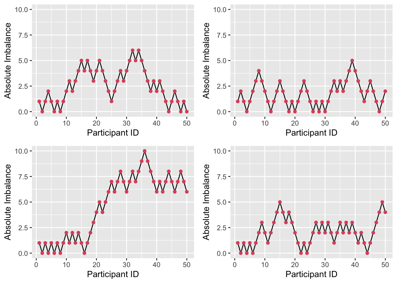
Figure 3.6: Four realisations of absolute imbalance for r=1, s=1, N=50.
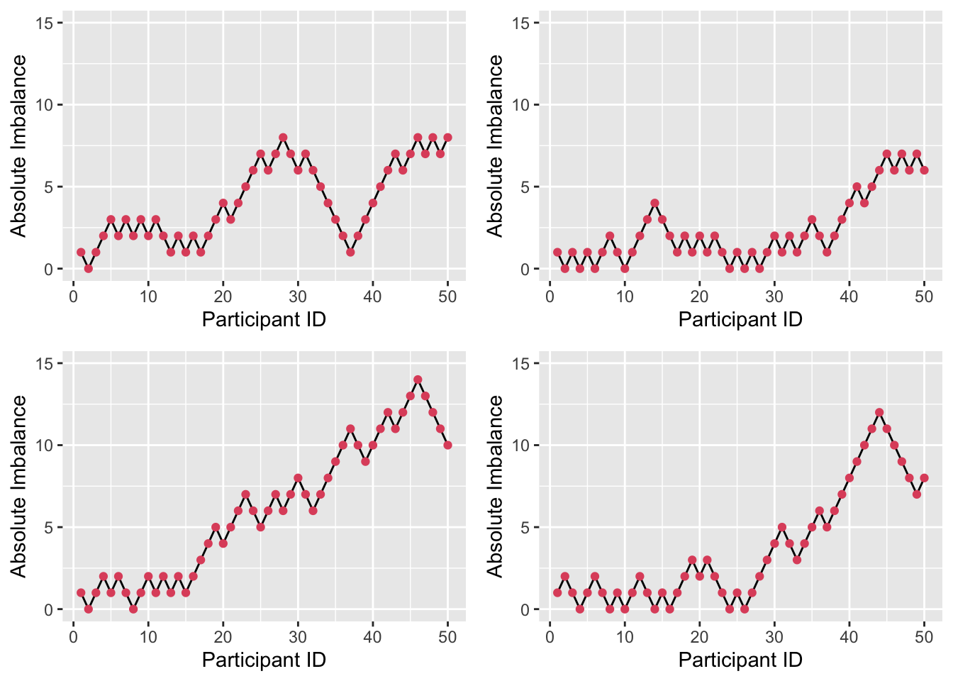
Figure 3.7: Four realisations of absolute imbalance for r=1, s=8, N=50.
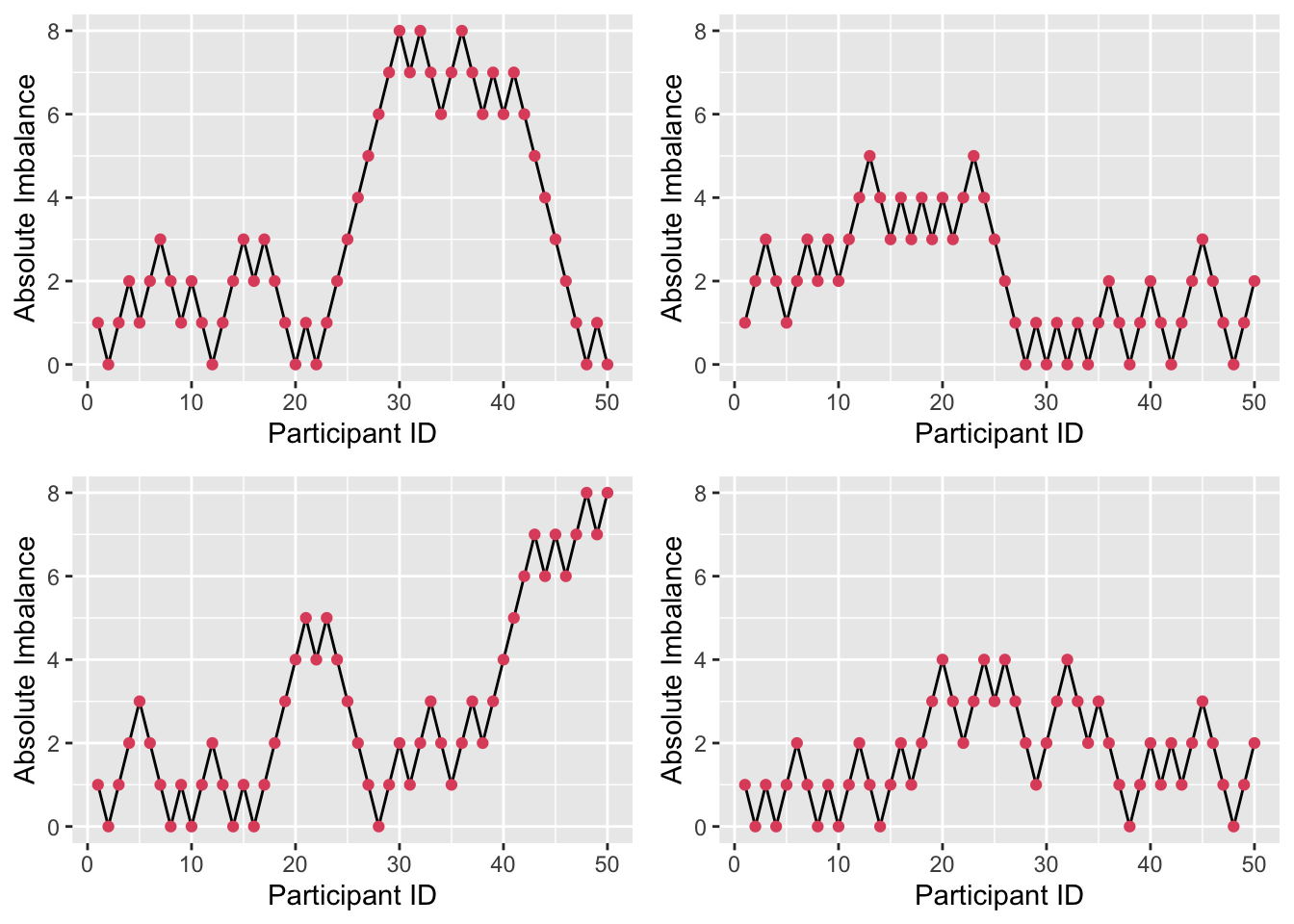
Figure 3.8: Four realisations of absolute imbalance for r=8, s=1, N=50.
We see that imbalance is reduced, particularly for small \(n\). A small \(r\) and large \(s\) enhance this, since the large number (\(s\)) of balls added to the urn with each allocation weight the probabilities more heavily, as in Figure 3.7. By contrast, if \(r\) is large and \(s\) is small, as in Figure 3.8, the probabilities stay closer to \(\left(\frac{1}{2}, \frac{1}{2}\right)\) and so more imbalance occurs early on.
3.3 Incorporating baseline measurements
At the start of the trial (ideally before allocation) various baseline measurements are usually taken. If the primary outcome variable is a continuous measurement (eg. blood pressure, weight,…) this same quantity will often be included, so that there is some measure of each participant’s condition/symptoms at the start of the trial. Factors such as age, sex, level of symptoms, things to do with treatment history and many others are included. Essentially, we include any variable we can that may lead to bias if not properly dealt with. The crucial thing is that none of these measurements (taken when they are) should be affected by the trial.
Such baseline measurements can be used in allocation.
3.3.1 Stratified sampling
The usual method of achieving balance with respect to prognostic factors is to divide each factor into several levels and to consider treatment assignment separately for patients having each particular combination of such factor levels. Such groups of patients are commonly referred to as randomization groups or strata. Treatment assignment is performed entirely separately for each stratum, a permuted block design of the type mentioned above often being used. In fact, using purely random treatment assignment for each stratum is equivalent to simple random assignment, so that some equalization of treatment numbers within each stratum is essential. Both the biased coin design and the urn design were intended for use in this way, adjusting in relation to imbalance within each stratum independently. This whole procedure is analogous to performing a factorial experiment, without being able to control the factor levels of the experimental units.
Example 3.5 Suppose we are planning a trial involving people over the age of 50, and we anticipate that age and sex might both play an important role in how participants respond to the treatment.
For sex, we use the levels ‘male’ and ‘female’, and for age we split the range into 50-65, 66-80 and 81 or over. We therefore have six strata, and we use an allocation strategy independently in each stratum. For example, below we have used randomly permuted blocks of length four.
| Male | Female | |
|---|---|---|
| 50-65 | ABAB BBAA … | ABBA BBAA … |
| 66-80 | BAAB AABB … | BABA BAAB … |
| 81 and over | ABAB ABBA … | ABBA BAAB … |
Each time a new participant arrives, we follow the randomization pattern for their stratum. We could use another allocation scheme within each stratum, for example an urn model or a biased coin. It is important that we use one that aims to conserve balance, or else the benefits of stratification are lost.
Example 3.6 The study by Kallis et al. (1994) compares the effect of giving aspirin to patients before coronary artery surgery with giving them a placebo. Interestingly, the effects of aspirin were found to be both positive (decreases platelet aggregation to arachidonic acid and to collagen) and negative (increased likelihood of post-operative excessive blood loss). For their prognostic factors, Kallis et al. (1994) chose age (\(\leq{50}\) or \(>50\)), sex (M or F), operating surgeon (3 possibilities) and number of coronary arteries affected (1 or 2). This creates 24 strata. The trial had 100 participants, meaning an average of 4.17 in each stratum.
A difficulty with stratified sampling is that the number of strata can quickly become large as the number of factors (or the number of levels within some factors) increases. For example, if we have four prognostic factors each with three levels, there are \(3^4=81\) strata. This creates a situation that is at best unwieldy, and at worst completely unworkable; in a small trial (with say 100 patients in each arm) there may be some strata with no patients in (this is actually not a problem), and probably many more with only one (this is much more problematic).
3.3.2 Minimization
Minimization was first proposed by Taves (1974), then shortly after by Pocock and Simon (1975) and Freedman and White (1976). The aim of minimization is to minimize the difference between the two groups. Although the method was developed in the seventies, it has only gained popularity relatively recently, mainly as computers have become widely available.
The people running the trial must first specify all of the factors they would like to be balanced between the two groups. These should be any variables that are thought to possibly affect the outcome.
When a patient enters the trial, their level of each factor is listed. The patient is then allocated in such a way as to minimise any difference in these factors between the two groups. The minimization method has evolved since its conception, and exists in several forms. Two areas in which methods vary are
- Whether continuous variables have to be binned
- Whether there is any randomness
It is generally agreed that if the risk of selection bias cannot be avoided, there should be an element of randomness. It is also usually accepted that if a variable is included in the minimization, it should also be included in the statistical analysis.
3.3.2.1 Minimization algorithm
Suppose we have a trial in which patients are recruited sequentially and need to be allocated to a trial arm (of which there are two). Pocock and Simon (1975) give an algorithm in the general case of \(N\) treatment arms, but we will not do that here.
Suppose there are several prognostic factors over which we require balance, and that these factors have \(I, J, K, ...\) levels. In the example above, there would be \(I=2,\; J=2,\; K=3,\; L=2\). Note that this equates to 24 strata.
At some point in the trial, suppose we have recruited \(n_{ijkl}\) patients with levels \(i,\,j,\,k,\,l\) of the factors. For example, this may be males, aged over 50, assigned to the second surgeon, with both coronary arteries affected. Within these, \(n^A_{ijkl}\) have been assigned to treatment arm \(A\), and \(n^B_{ijkl}\) to arm \(B\). So we have
\[ n^A_{ijkl} + n^B_{ijkl} = n_{ijkl} .\]
If we were to use random permuted blocks within each stratum, then we would be assured that
\[\lvert n^A_{ijkl} - n^B_{ijkl} \rvert \leq{\frac{1}{2}b},\] where \(b\) is the block length. However, there are two issues with this:
- There may be very few patients in some strata, in which case RPBs will fail to provide adequate balance.
- It is unlikely that we actually need this level of balance.
The first point is a pragmatic one - the method usually guaranteed to achieve good balance is likely to fail, at least for some strata. The second is more theoretical. In general, we require that groups be balanced according to each individual prognostic factor, but not to interactions. For example, it is often believed that younger patients would have generally better outcomes, but that other factors do not systematically affect this difference.
Therefore, it is enough to make sure that the following are all small:
\[ \begin{aligned} \lvert n^A_{i+++} - n^B_{i+++} \rvert&\text{ for each }i=1,\ldots,I\\ \lvert n^A_{+j++} - n^B_{+j++} \rvert&\text{ for each }j=1,\ldots,J\\ \ldots& \end{aligned} \] where \(+\) represents summation over the other factors, so that for example
\[n^A_{++k+} = \sum\limits_{i,j,l}{n^A_{ijkl}}\] is the total number of patients with level \(k\) of that factor assigned to treatment arm \(A\).
Therefore, instead of having \(IJKL\) constraints constraints, as we would with using randomly permuted blocks (or some other randomization method) within each stratum, we have \(I+J+K+L\) constraints, one for each level of each factor. In our example this is 9 constraints rather than 24.
In order to implement minimisation, we follow these steps:
- Allocate the first patient by simple randomisation.
- Suppose that at some point in the trial we have recruited \(n_{ijkl}\) patients with prognostic factors \(i,\,j,\,k,\,l\). Of these \(n^A_{ijkl}\) are allocated to treatment arm \(A\) and \(n^B_{ijkl}\) to arm \(B\).
- A new patient enters the trial. They have prognostic factors at levels \(w,\,x,\,y,\,z\).
- We form the sum
\[\begin{equation} \left(n^A_{w+++} - n^B_{w+++}\right) + \left(n^A_{+x++} - n^B_{+x++}\right) + \left(n^A_{++y+} - n^B_{++y+}\right) + \left(n^A_{+++z} - n^B_{+++z}\right). \tag{3.1} \end{equation}\]
- If the sum from step 4 is negative (that is, allocation to arm \(B\) has dominated up to now) then we allocate the new patient to arm \(A\) with probability \(P\), with \(P>0.5\). If the sum is positive, they are allocated to arm \(B\) with probability \(P\). If the sum is zero, they are allocated to arm \(A\) with probability \(\frac{1}{2}\).
Some people set \(P=1\), whereas others would set \(\frac{1}{2}<P<1\) to retain some randomness. Although setting \(P=1\) makes the system deterministic, to predict the next allocation a doctor (or whoever) would need to know \(n^A_{i+++}\) and so on. This is very unlikely unless they are deliberately seeking to disrupt the trial. However, generally the accepted approach is becoming to set \(P<1\).
Example 3.7 From Altman (1990) (citing Fentiman, Rubens, and Hayward (1983)). In this trial, 46 patients with breast cancer were allocated to receive either Mustine (arm A) or Talc (arm B) as treatment for pleural effusions (fluid between the walls of the lung). They used four prognostic factors: age (\(\leq{50}\) or \(>50\)), stage of disease (I or II, III or IV), time in months between diagnosis of breast cancer and diagnosis of pleural effusions (\(\leq{30}\) or \(>30\)) and menopausal status (Pre or post).
Let’s suppose that 15 patients have already been allocated. The totals of patients in each treatment arm in terms of each level of each prognostic factor are shown in the table below.
| factor | level | Mustine (A) | Talc (B) |
|---|---|---|---|
| Age | 1. 50 or younger | 3 | 4 |
| Age | 2. >50 | 4 | 4 |
| Stage | 1. I or II | 1 | 2 |
| Stage | 2. III or IV | 6 | 6 |
| Time interval | 1. 30 months or less | 4 | 2 |
| Time interval | 2. >30 months | 4 | 5 |
| Menopausal status | 1. Pre | 4 | 3 |
| Menopausal status | 2. Post | 5 | 3 |
Suppose our sixteenth patient is under 50, has disease at stage III, has less than 30 months between diagnoses and is pre-menopausal. Our calculation from step 4 of the minimisation algorithm is therefore
\[ \begin{aligned} \left(n^A_{1+++} - n^B_{1+++}\right) + \left(n^A_{+2++} - n^B_{+2++}\right) + \left(n^A_{++1+} \right.& \left.- n^B_{++1+}\right) + \left(n^A_{+++1} - n^B_{+++1}\right) \\ & = \left(3-4\right) + \left(6-6\right) + \left(4-2\right) + \left(4-3\right) \\ & = -1 + 0 + 2 + 1\\ & = 2 . \end{aligned} \] Since our sum is greater than zero, we allocate the new patient to arm B (talc) with some probability \(P\in\left(0.5,1\right)\) and update the table before allocating patient 17.
One shortcoming of minimisation is that the factors are equally weighted in the algorithm, regardless of the number of patients with that particular factor level. For example, suppose at some later stage of allocation in our Mustine example, only four patients with stage I or II disease had been recruited, and that one of these had been allocated to group \(A\) and three to group \(B\). At the same point, 18 of the recruited number were post-menopausal, and of these 10 had been allocated to group \(A\) and 8 to group \(B\). The values contributed to the sum in Equation (3.1) are \(+2\) and \(-2\), so these imbalances effectively cancel one another out, but intuitively it would feel sensible to prioritise equal distribution within the stage I or II women, since proportionally this stratum is less balanced. Wei (1978) proposed an extension of the Urn Design that does exactly this, but we won’t cover this method in our course.
3.4 Problems around allocation
In clinical trials papers, the allocation groups are usually summarised in tables giving summary statistics (eg. mean and SD) of each characteristic for the control group and the intervention group. The aim of these is to show that the groups are similar enough for any difference in outcome to be attributed to the intervention itself. Figure 3.9 shows an example, taken from Ruetzler et al. (2013).
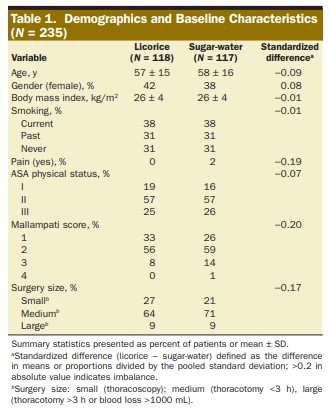
Figure 3.9: Summary statistics for an RCT comparing a licorice gargle (the intervention) to a sugar-water gargle (the standard). From Ruetzler et al. (2013)
An issue here is that only the marginal distributions are compared for similarity. Consider the following (somewhat extreme and minimalistic) scenario. A study aims to investigate the effect of some treatment, and to balance for gender and age in their allocation, resulting in the following summary table.
| Male | Female | |
|---|---|---|
| Control | 57.51 (7.09) | 40.31 (5.83) |
| Intervention | 44.19 (5.96) | 60.03 (5.27) |
This appears to be a reasonably balanced design. However, if we look at the joint distribution, we see that there are problems.
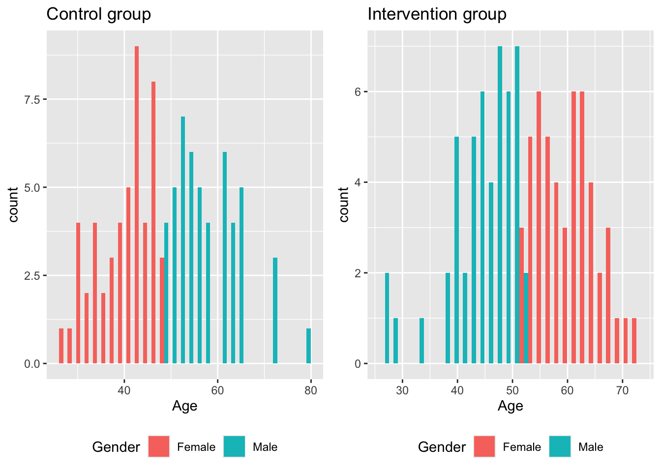
If the intervention is particularly effective in older men, our trial will not notice. Likewise, if older women generally have a more positive outcome than older men, our trial may erroneously find the intervention to be effective.
Although this example is highly manufactured and [hopefully!] unlikely to take place in real life, for clinical trials there are often many demographic variables and prognostic factors being taken into account. Achieving joint balance across all them is very difficult, and extremely unlikely to happen if it isn’t aimed for. Treasure and MacRae (1998) give an example in relation to a hypothetical study on heart disease
Supposing one group has more elderly women with diabetes and symptoms of heart failure. It would then be impossible to attribute a better outcome in the other group to the beneficial effects of treatment since poor left ventricular function and age at outset are major determinants of survival in any longitudinal study of heart disease, and women with diabetes, as a group, are likely to do worse. At this point the primary objective of randomisation—exclusion of confounding factors—has failed. … If a very big trial fails, because, for example, the play of chance put more hypertensive smokers in one group than the other, the tragedy for the trialists, and all involved, is even greater.
However, this issue is rarely addressed in clinical trials: a lot of faith is placed (with reasonable justification) in the likely balance achieved by random sampling, whatever method is used. We will also see in the next Chapter that we can account for some degree of imbalance at the analysis stage.