4 Analyzing RCT data
We’re now in the post-trial stage. The trial has been run, and we have lots of data to analyze to try to assess what effect the treatment or intervention has had. In general we will use the notation \(\tau\) to denote the treatment effect.
In this chapter we’ll keep our focus on the scenario where the trial outcome is measured on a continuous scale, but in later weeks we’ll go on to look at other types of data.
Example 4.1 To illustrate the theory and methods, we’ll use an example dataset from Hommel et al. (1986) (this example is also used by Matthews (2006)). The data involves a trial of 16 diabetes patients, and focusses on a drug (Captopril) that may reduce blood pressure. This is important, since for those with diabetes, high blood pressure can exacerbate kidney disease (specifically diabetic nephropathy, a complication of diabetes). To participate in the trial, people had to be insulin-dependent and already affected by diabetic nephropathy. In the trial, systolic blood pressure (the primary outcome) was measured before participants were allocated to each trial arm, and then measured again after one week on treatment. A placebo was given to the control group, so that all participants were blinded.
The baseline and outcome blood pressure measurements (in mmHg) are shown in Table 4.1. We see that nine participants were assigned to the treatment arm (Captopril) and the remaining seven to the placebo group. Hommel et al. (1986) say that the patients were ‘randomly allocated’ to their group.
| Patient (ID) | Baseline (B) | Outcome at 1 week (X) | Trial Arm |
|---|---|---|---|
| 1 | 147 | 137 | Captopril |
| 2 | 129 | 120 | Captopril |
| 3 | 158 | 141 | Captopril |
| 4 | 164 | 137 | Captopril |
| 5 | 134 | 140 | Captopril |
| 6 | 155 | 144 | Captopril |
| 7 | 151 | 134 | Captopril |
| 8 | 141 | 123 | Captopril |
| 9 | 153 | 142 | Captopril |
| 1 | 133 | 139 | Placebo |
| 2 | 129 | 134 | Placebo |
| 3 | 152 | 136 | Placebo |
| 4 | 161 | 151 | Placebo |
| 5 | 154 | 147 | Placebo |
| 6 | 141 | 137 | Placebo |
| 7 | 156 | 149 | Placebo |
This is very small dataset, and so in that respect it is quite unusual, but its structure is similar to many other trials.
We will build up from the simplest type of analysis to some more complicated / sophisticated approaches.
4.1 Confidence intervals and P-values
Because the randomization process should produce groups that are comparable, we should in principle be able to compare the primary outcome (which we’ll still denote \(X\)) between the groups.
Example 4.2 Summary statistics of the outcome for each group are shown in Table 4.2.
| Sample Size | Mean (mmHg) | SD (mmHg) | SE of mean (mmHg) | |
|---|---|---|---|---|
| Captopril | 9 | 135.33 | 8.43 | 2.81 |
| Placebo | 7 | 141.86 | 6.94 | 2.62 |
We see that the difference in mean outcome (systolic blood pressure) between the two groups is \(141.86 - 135.33 = 6.53 \text{mmHg}\). Clearly overall there has been some reduction in systolic blood pressure for those in the Captopril arm, but how statistically sound is this as evidence? It could be that really (for the wider population) there is no reduction, and we have just been ‘lucky’.
The variances within the two groups are fairly close, so we can use the pooled estimate of standard deviation:
\[ s_p = \sqrt{\frac{\sum\limits_{i=1}^N\left(n_i-1\right)s_i^2}{\sum\limits_{i-1}^N\left(n_i-1\right)}}. \]
In our case
\[ \begin{aligned} s_p&= \sqrt{\frac{8\times{8.43^2} + 6 \times{6.94^2}}{8+6}}\\ & = 7.82\text{ mmHg.} \end{aligned} \] This enables us to do an independent two-sample \(t\)-test, by computing the standardized measure of effect size we found in Section 2.3. We find the test statistic
\[ \begin{aligned} D & = \frac{\bar{X_C} - \bar{X_T}}{s_p\sqrt{\frac{1}{n_C} + \frac{1}{n_T}}}\\ & = \frac{6.53}{7.82\sqrt{\frac{1}{7} + \frac{1}{9}}} \\ & = 1.65. \end{aligned} \] Note that here the placebo group is group \(C\), and the Captopril group is group \(T\).
Under the null hypothesis that the mean systolic blood pressure at the end of the week of treatment/placebo is the same in both groups, this value should have a \(t\) distribution with 14 degrees of freedom (\(n_i-1\) for each group).
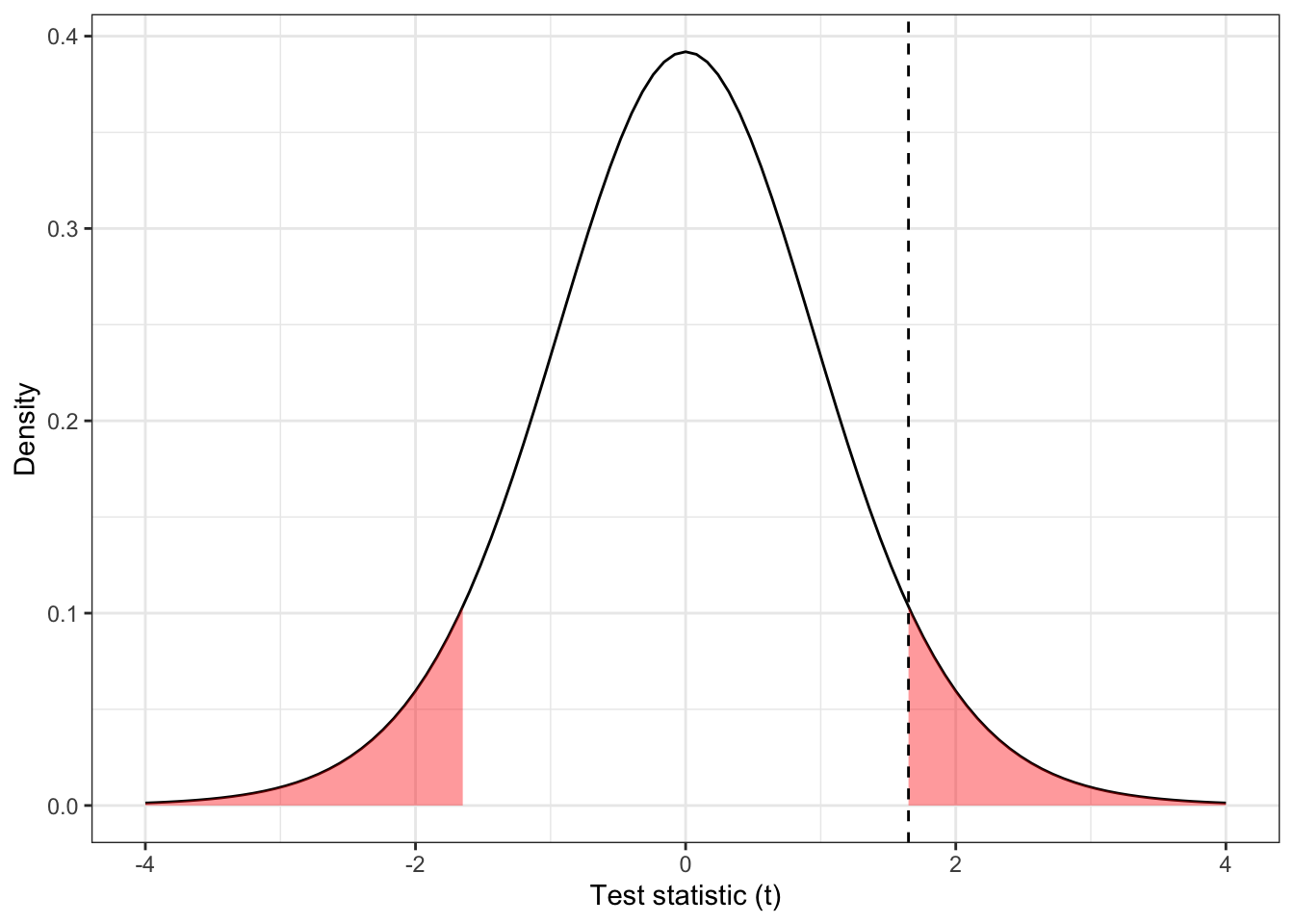
Figure 4.1: The distribution \(t_{14}\), with \(D=1.65\) shown by the dashed line and the ‘more extreme’ areas shaded.
The dashed line in Figure 4.1 is at \(D=1.65\), and the red shaded areas show anywhere ‘at least as extreme’. We can find the area (ie. the probability of anything at least as extreme as our found value) in R by
## [1] 0.1211902This is the value we know as ‘the P value’. We see that in this case our results are not statistically significant (even at the 0.10 level), under this model.
4.1.1 What do we do with this outcome?
The outcome of this Captopril study is in some ways the worst case scenario. The difference in means is large enough to be compelling, but our dataset is too small for it to be statistically significant, and so we can’t confidently conclude that Captopril has any effect on blood pressure. However, we also can’t say that there is no effect. This is exactly the sort of scenario we hoped to avoid when planning our study.
One way to reframe the question is to consider the range of treatment effects that are compatible with our trial data. That is, we find the set
\[\left\lbrace \tau \mid \frac{\lvert \bar{x}_C - \bar{x}_T - \tau \rvert}{s\sqrt{n_C^{-1} + n_T^{-1}}} \leq t_{n_C+n_T-2;\,0.975} \right\rbrace, \] which contains all possible values of treatment effect \(\tau\) that are compatible with our data. That is, suppose the true treatment effect is \(\tau^*\), and we test the hypothesis that \(\tau = \tau^*\). For all values of \(\tau^*\) inside this range, our data are not sufficiently unlikely to reject the hypothesis at the 0.05 level. However, for all values of \(\tau^*\) outside this range, our data are sufficiently unlikely to reject that hypothesis. We can rearrange this to give a 95% confidence interval for \(\tau\),
\[\left\lbrace \tau \mid \bar{x}_C - \bar{x}_T - t_{n_C+n_T-2;\,0.975}\,s\sqrt{n_C^{-1} + n_T^{-1}} \leq \tau \leq \bar{x}_C - \bar{x}_T + t_{n_C+n_T-2;\,0.975}\,s\sqrt{n_C^{-1} + n_T^{-1}} \right\rbrace \]
Example 4.3 Continuing our example, we have
\[\left\lbrace \tau \mid \frac{\lvert 6.53 - \tau \rvert}{7.82\sqrt{\frac{1}{7} + \frac{1}{9}}} \leq t_{14;0.975} = 2.145 \right\rbrace \]
Here, \(t_{14;0.975} = 2.145\) is the \(t\)-value for a significance level of \(0.05\), so if we were working to a different significance level we would change this.
Rearranging as above, this works out to be the interval
\[ -1.92 \leq \tau \leq 14.98. \]
Notice that zero is in this interval, consistent with the fact that we failed to reject the null hypothesis.
Some things to note
- We can compute this confidence interval whether or not we failed to reject the null hypothesis that \(\tau=0\), and for significance levels other than 0.05.
- In most cases, reporting the confidence interval is much more informative than simply reporting the \(P\)-value. In our Captopril example, we found that a negative treatment effect (ie. Captopril reducing blood pressure less than the placebo) of more than 2 mmHg was very unlikely, whereas a positive effective (Captopril reducing blood pressure) of up to 15 mmHg was plausible. If Captopril were inexpensive and had very limited side effects (sadly neither of which is true) it may still be an attractive drug.
- These confidence intervals are exactly the same as you have learned before, but we emphasise them because they are very informative in randomised controlled trials (but not so often used!).
At the post trial stage, when we have data, the confidence interval is the most useful link to the concept of power, which we thought about at the planning stage. Remember that the power function is defined as
\[\psi \left(\tau\right) = P\left(\text{Reject }H_0\mid \tau\neq 0\right),\] that is, the probability that we successfully reject \(H_0\) (that \(\tau=0\)) given that there is a non-zero treatment effect \(\tau\neq 0\). This was calculated in terms of the theoretical model of the trial, and in terms of some minimum detectable effect size \(\tau_M\) that we wanted to be able to correctly detect with probability \(1-\beta\) (the power). It is difficult to say anything meaningful about the power of a trial after the fact. That said, if we failed to reject \(H_0\) and \(\tau_M\) is in the confidence interval for \(\tau\), then that is a good indication that our trial was indeed underpowered.
4.2 Using baseline values
In the example above, our primary outcome variable \(X\) was the systolic blood pressure of each participant at the end of the intervention period. However, we see in Table 4.1 that we also have baseline measurements: measurements of systolic blood pressure for each patient from before allocation (and therefore before they received the treatment or placebo). Baseline measurements are useful primarily for two reasons:
- They can be used to assess the balance of the design.
- They can be used in the analysis.
We will demonstrate these by returning to our Captopril example.
Example 4.4 Firstly, we use the baseline systolic blood pressure to assess balance. The placebo group has a mean of 146.6 mmHg and an SD of 12.3 mmHg, whereas the Captopril group has mean 148.0 mmHg, SD 11.4 mmHg. While these aren’t identical, they are sufficiently similar not to suspect any systematic imbalance. In a study this small there is likely to be some difference.
Secondly, since we are interested in whether the use of Captopril has reduced blood pressure for each individual, and these individuals had different baseline values, it makes sense to compare not just the outcome but the difference from baseline to outcome for each individual. We can see individual data in Table 4.3 and summary statistics in Table 4.4.
| Patient (ID) | Baseline (B) | Outcome at 1 week (X) | Trial Arm | Difference |
|---|---|---|---|---|
| 1 | 147 | 137 | Captopril | -10 |
| 2 | 129 | 120 | Captopril | -9 |
| 3 | 158 | 141 | Captopril | -17 |
| 4 | 164 | 137 | Captopril | -27 |
| 5 | 134 | 140 | Captopril | 6 |
| 6 | 155 | 144 | Captopril | -11 |
| 7 | 151 | 134 | Captopril | -17 |
| 8 | 141 | 123 | Captopril | -18 |
| 9 | 153 | 142 | Captopril | -11 |
| 1 | 133 | 139 | Placebo | 6 |
| 2 | 129 | 134 | Placebo | 5 |
| 3 | 152 | 136 | Placebo | -16 |
| 4 | 161 | 151 | Placebo | -10 |
| 5 | 154 | 147 | Placebo | -7 |
| 6 | 141 | 137 | Placebo | -4 |
| 7 | 156 | 149 | Placebo | -7 |
| Sample Size | Mean (mmHg) | SD (mmHg) | SE of mean (mmHg) | |
|---|---|---|---|---|
| Captopril | 9 | -12.67 | 8.99 | 3.00 |
| Placebo | 7 | -4.71 | 7.91 | 2.99 |
We can perform an unpaired t-test as before, in which case we find
\[ t = \frac{-4.71 - (-12.67)}{8.54\sqrt{\frac{1}{7}+\frac{1}{9}}} = 1.850 \] where 8.54 is the pooled standard deviation. Under the null hypothesis of no difference, this test statistic has a \(t\)-distribution with 14 degrees of freedom, and so we have a \(P\)-value of 0.086.
## [1] 0.08553164Our 0.95 confidence interval is
\[\underbrace{-4.71 - (-12.67)}_{\text{Mean difference}} \pm t_{14;\,0.975}\times \underbrace{8.54\sqrt{\frac{1}{7}+\frac{1}{9}}}_{\text{Pooled SD}} = \left[-1.3,\,17.2\right].\] We see that taking into account the baseline values in this way has slightly reduced the \(P\)-value and shifted the confidence interval slightly higher. Though at the \(\alpha = 0.05\) level we still don’t have significance.
We will now look into why the confidence interval and \(P\)-value changed in this way, before going on to another way of taking into account the baseline value.
4.2.1 The variance of the treatment effect estimate
Let’s label the baseline measurement for each group \(B_C\) and \(B_T\), and the outcome measurements \(X_C,\,X_T\), where we will take group \(C\) to be the placebo/control group and group \(T\) to be the treatment group. Because all participants have been randomised from the same population, we have
\[\operatorname{E}\left(B_C\right) = \operatorname{E}\left(B_T\right) = \mu_B.\] Assuming some treatment effect \(\tau\) (which could still be zero) we have
\[ \begin{aligned} \operatorname{E}\left(X_C\right) & = \mu\\ \operatorname{E}\left(X_T\right) & = \mu + \tau. \end{aligned} \] Usually we will assume that
\[\operatorname{Var}\left(X_C\right) = \operatorname{Var}\left(X_T\right) = \operatorname{Var}\left(B_C\right) = \operatorname{Var}\left(B_T\right) = \sigma^2,\] and this is generally fairly reasonable in practice.
Notice that for the two analyses we have performed so far (comparing outcomes and comparing outcome-baseline differences) we have
\[ \begin{aligned} \operatorname{E}\left(X_T\right) - \operatorname{E}\left(X_C\right) & = \left(\mu + \tau\right) - \mu = \tau\\ \operatorname{E}\left(X_T - B_T\right) - \operatorname{E}\left(X_C - B_C\right) & = \left(\mu - \mu_B + \tau\right) - \left(\mu - \mu_B\right) = \tau, \end{aligned} \] that is, both are unbiased estimators of \(\tau\).
However, whereas the first is based on data with variance \(\sigma^2\), the second has
\[ \begin{aligned} \operatorname{Var}\left(X_T-B_T\right) & = \operatorname{Var}\left(X_T\right) + \operatorname{Var}\left(B_T\right) - 2\operatorname{cov}\left(X_T,B_T\right)\\ & = \sigma^2 + \sigma^2 - 2\rho\sigma^2 \\ & = 2\sigma^2\left(1-\rho\right), \end{aligned} \] where \(\rho\) is the true correlation between \(X\) and \(B\), and is assumed to be the same in either group. Similarly,
\[\operatorname{var}\left(X_C-B_C\right) = 2\sigma^2\left(1-\rho\right).\]
Using this to work out the variance of the estimators we find that for comparing means, assuming two equally sized groups of size \(N\), we have
\[\operatorname{var}\left(\hat{\tau}_{\text{out}}\right) = \operatorname{var}\left(\bar{x}_T - \bar{x}_C\right) = \frac{2\sigma^2}{N}.\]
whereas for comparing differences from baseline
\[\operatorname{var}\left(\hat{\tau}_{\text{diff}}\right) = \operatorname{var}\left[\left(\overline{X_T-B_T}\right) - \left(\overline{X_C - B_C}\right)\right] = 2\left(1-\rho\right)\left(\frac{2\sigma^2}{N}\right).\]
Therefore, if \(\frac{1}{2}<\rho\leq 1\) there will be a smaller variance when comparing differences than when using just the outcome variable. However, if \(\rho<\frac{1}{2}\), the variance will be smaller when comparing outcome variables.
Intuitively, this seems reasonable: if the correlation between baseline and outcome measurements is very strong, then we can remove some of the variability between participants by taking into account their baseline measurement. However, if the correlation is weak, then by including the baseline in the analysis we are essentially just introducing noise. If the correlation is negative (very unusual in practice) then \(\operatorname{var}\left(\hat{\tau}_{\text{diff}}\right)\) is much larger than \(\operatorname{var}\left(\hat{\tau}_{\text{out}}\right)\) - this also makes sense intuitively because we aren’t allowing the coefficient of the baseline measurement to reflect the relationship between baseline and outcome.
Example 4.5 For our Captopril example, the sample correlation between baseline and outcome is 0.63 in the Captopril group and 0.80 in the Placebo group. This fits with the \(P\)-value having reduced slightly.
4.2.2 A dodgy way to use baseline variables
Sometimes the analysis performed on a dataset is rather spurious, but it isn’t always immediately obvious why. We’ll look at one example now, because it is sometimes done.
This approach involves looking at each group separately, and determining whether there has been a significant change in the outcome variable (note that this only ‘works’ if \(\mu_B = \mu\), ie. if you wouldn’t expect a change in \(X\) over time anyway). One thing that makes this analysis attractive is that it lends itself to a paired \(t\)-test, which is more poweful (in general).
Example 4.6 Returning to our Captopril data, we could perform a paired \(t\)-test on the difference between baseline \(B\) and outcome \(X\) for each patient, for each group.
If we do this, we find the summary statistics in Table 4.5.
| T statistic | Deg of freedom | P-value | |
|---|---|---|---|
| Captopril | 4.23 | 8 | 0.003 |
| Placebo | 1.58 | 6 | 0.170 |
From this we see that there is strong evidence for a change in blood pressure for the Captopril patients (group \(T\)), which isn’t surprising, and no such evidence for the placebo patients. Can we therefore conclude that Captopril is significantly better than the placebo? No! The analysis is flawed:
- The \(p\)-value of 0.17 in the control group doesn’t show that the null hypothesis (no treatment effect for the control group) is true, just that we can’t reject the null hypothesis. It is quite possible that there is a difference in the control group, and that numerically it could even be comparable to that in the treatment group, so although we can say that there is a significant reduction in blood pressure for the captopril group, we can’t conclude that Captopril is better than the placebo.
- Having set up the experiment as a randomised controlled trial, with a view to comparing the two groups, it seems strange to then deal with them separately.
4.3 Analysis of covariance (ANCOVA)
In the previous section we based our analysis on the baseline values being statistically identical draws from the underlying distribution, and therefore having the same expectation and variance.
However, although this is theoretically true, in real life trials there will be some imbalance in the baseline measurements for the different treatment arms. We can see this in our Captopril example, in Figure 4.2.
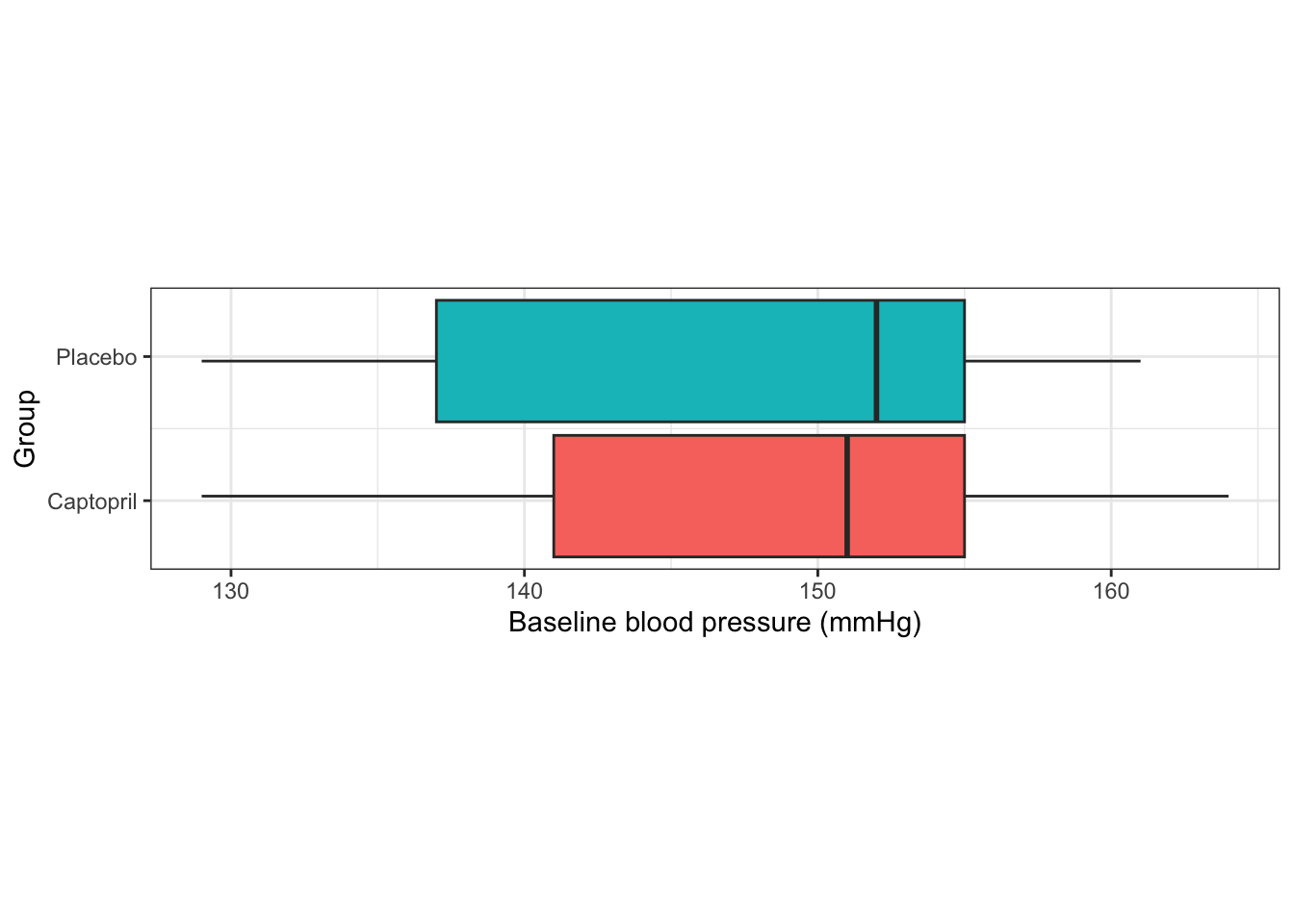
Figure 4.2: Baseline measurements from the Captopril trial.
The baseline measurements are not identical in each group. Indeed, we saw earlier that the means differ by 1.4 mmHg. Although this isn’t a clinically significant difference, or a large enough difference to make us doubt the randomisation procedure, it is still a difference.
The basic principle of ANCOVA is that if there is some correlation between the baseline and outcome measurements, then if the baseline measurements differ, one would expect the outcome measurements to differ, even if there is no treatment effect (ie. if \(\tau=0\)). Indeed, how do we decide how much of the difference in outcome is down to the treatment itself, and how much is simply the difference arising from different samples?
This issue arises in many trials, particularly where there is a strong correlation between baseline and outcome measurements.
4.3.1 The theory
Suppose the outcome for a clinical trial is \(X\), which has mean \(\mu\) in the control group (C) and mean \(\mu+\tau\) in the treatment group (T), and as usual our aim is to determine the extent of \(\tau\), the treatment effect. We suppose also that \(X\) has variance \(\sigma^2\) in both groups.
The same quantity is measured at the start of the trial, and this is the baseline \(B\), which we can assume to have true mean \(\mu_B\) in both groups (because of randomisation) and variance \(\sigma^2\). We also assume that the true correlation between \(B\) and \(X\) is \(\rho\) in each group. Finally, we assume that both trial arms are of size \(N\). We therefore have \(2N\) patients, and so we observe baseline measurements \(b_1,\,b_2,\ldots,b_{2N}\).
Our first step is to find an estimator for \(\tau\) that uses this information.
4.3.1.1 Finding an estimator
Let’s suppose that random variables \(Z\) and \(Y\) are jointly normally distributed with correlation \(\rho\)
\[\begin{equation} \begin{pmatrix} Z\\ Y \end{pmatrix} \sim N\left( \begin{pmatrix} \mu_Z\\ \mu_Y \end{pmatrix},\; \begin{pmatrix} \sigma^2_Z & \rho\sigma_Z\sigma_Y \\ \rho\sigma_Z\sigma_Y & \sigma^2_Y \end{pmatrix} \right). \tag{4.1} \end{equation}\]
From Equation (4.1), we know that \(\operatorname{E}\left(Y\right) = \mu_Y\).
But, if we have observed \(Z=z\), this gives us some information about likely values of \(Y\): if \(\rho>0\) then a lower value of \(z\) should lead us to expect a lower value of \(Y\), for example. Figure 4.3 shows
\[\begin{equation} \begin{pmatrix} Z\\ Y \end{pmatrix} \sim N\left( \begin{pmatrix} 0\\ 0 \end{pmatrix},\; \begin{pmatrix} 2 & 1.5 \\ 1.5 & 3 \end{pmatrix} \right). \tag{4.2} \end{equation}\]
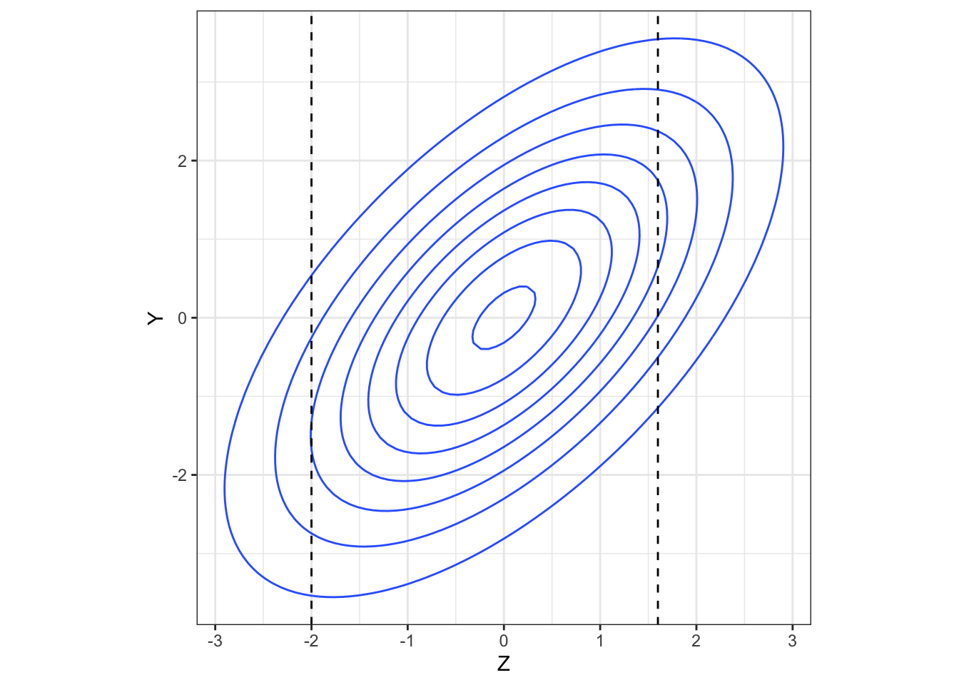
Figure 4.3: A bivariate normal density.
The higher the value of \(\rho\) (in magnitude), the more the conditional distribution of \(Y\) given an observed value of \(z\) deviates from the marginal distribution of \(Y\) (in our example, \(N\left(0,\;3\right)\)). In particular, \[\operatorname{E}\left(Y\mid{Z=z}\right)\neq{\operatorname{E}\left(Y\right)}.\]
If we have another random variable, \(W\), that is independent of \(Y\) (and note that if two normally distributed variables are uncorrelated, they are also independent), then observing \(W=w\) doesn’t give us any information about the distribution of \(Y\), so we have
\[ \operatorname{E}\left(Y\mid{W=w}\right)={\operatorname{E}\left(Y\right)}. \] We can combine this information to work out \(\operatorname{E}\left(Y\mid{Z=z}\right)\). Firstly, we’ll calculate the covariance of \(Z\) and \(Y-kZ\), for some constant \(k\). We can find this by
\[ \begin{aligned} \operatorname{cov}\left(Z,\,Y-kZ\right) &= \operatorname{E}\big[\left(Z-\mu_Z\right)\left(Y-kZ - \mu_Y + k\mu_Z\right)\big]\\ &\text{ (using that }\operatorname{cov\left(Z,Y\right)=\operatorname{E}\left[\left(Z-\operatorname{E}\left(Z\right)\right)\left(Y-\operatorname{E}\left(Y\right)\right)\right]}\\ & = \operatorname{E}\left[\left(Z-\mu_Z\right)\left(Y-\mu_Y\right) - k\left(Z-\mu_Z\right)^2\right]\\ & = \rho \sigma_Z\sigma_Y - k\sigma_Z^2. \end{aligned} \] If we set
\[k = \beta = \frac{\rho\sigma_Y}{\sigma_Z} \] then \(\operatorname{cov}\left(Z,\,Y-\beta Z\right)=0\), and since \(Y-\beta Z\) is also normally distributed, this means that \(Z\) and \(Y-\beta Z\) are independent. Therefore we have
\[\operatorname{E}\left(Y-\beta Z \mid Z=z\right) = \operatorname{E}\left(Y-\beta Z\right) = \mu_Y - \beta \mu_Z.\]
However, since we’re conditioning on an observed value of \(Z=z\) we can take \(Z\) to be fixed at this value, and so \(\operatorname{E}\left(\beta Z\mid{Z=z}\right) = \beta z\). Finally, this allows us to calculate
\[ \begin{aligned} \operatorname{E}\left(Y\mid{Z=z}\right) & = \operatorname{E}\left(\beta Z\mid{Z=z}\right) + \mu_Y - \beta\mu_Z\\ & = \mu_Y + \beta\left(z - \mu_Z\right). \end{aligned} \]
We can apply this to our clinical trials setting to find
\[ \begin{aligned} \operatorname{E}\left(X_i\mid{b_i}\right) &= \mu + \rho\left(b_i - \mu_B\right)\text{ in the control group}\\ \operatorname{E}\left(X_i\mid{b_i}\right) &= \mu +\tau + \rho\left(b_i - \mu_B\right)\text{ in the test group.} \end{aligned} \] Notice that because in our model \(\sigma_T = \sigma_C = \sigma\), we have \(\beta = \rho\).
From this, we find that
\[\begin{equation} \operatorname{E}\left(\bar{X}_T - \bar{X}_C\mid{\bar{b}_T,\,\bar{b}_C}\right) = \tau + \rho\left(\bar{b}_T - \bar{b}_C\right). \tag{4.3} \end{equation}\] That is, if there is a difference in the baseline mean between the control and test groups, then the difference in outcome means is not an unbiased estimator of the treatment effect \(\tau\). Assuming \(\rho>0\) (which is almost always the case) then if \(\bar{b}_T>\bar{b}_C\) the difference in outcome means overestimates \(\tau\). Conversely, if \(\bar{b}_T<\bar{b}_C\), the difference in outcome means underestimates \(\tau\). The only situation in which the difference in outcome means is an unbiased estimator is when \(\rho=0\), however this is not common in practice.
Comparing the difference between outcome and baseline, as we did in 4.2, does not solve this problem, since we have
\[\operatorname{E}\left[\left(\bar{X}_T - \bar{b}_T\right) - \left(\bar{X}_C - \bar{b}_C\right)\mid{\bar{b}_T,\,\bar{b}_C}\right] = \tau + \left(\rho-1\right)\left(\bar{b}_T - \bar{b}_C\right),\] which is similarly biased (unless \(\rho=1\), which is never the case).
Notice, however, that if we use as our estimator
\[\begin{equation} \hat{\tau} = \left(\bar{X}_T - \bar{X}_C\right) - \rho \left(\bar{b}_T - \bar{b}_C\right) \tag{4.4} \end{equation}\]
then, following from Equation (4.3) we have
\[ \operatorname{E}\left[\left(\bar{X}_T - \bar{X}_C\right) - \rho \left(\bar{b}_T - \bar{b}_C\right)\mid{\bar{b}_T,\,\bar{b}_C}\right] = \tau + \rho\left(\bar{b}_T - \bar{b}_C\right)- \rho\left(\bar{b}_T - \bar{b}_C\right) = \tau. \]
We now return to our general bivariate normal variables \(Y\) and \(Z\) to find the variance of this estimator.
4.3.1.2 What’s the variance of this estimator?
To work out the variance of \(\hat{\tau}\) in Equation (4.4) we need to go back to our bivariate normal variables.
Recall that \(\operatorname{var}\left(Y\right) = \operatorname{E}\left[Y^2\right] - \left[\operatorname{E}\left(Y\right)\right]^2\), and so
\[\begin{equation} \operatorname{var}\left(Y\mid{Z=z}\right) = \operatorname{E}\left(Y^2\mid{Z=z}\right) - \left[\operatorname{E}\left(Y\mid{Z=z}\right)\right]^2. \tag{4.5} \end{equation}\]
We already know the second term, and we can find the first term using the same idea as before, this time noting that \(Z\) and \(\left(Y-\beta Z\right)^2\) are independent.
From this, and using the fact that (for example)
\[ \begin{aligned} \operatorname{var}\left(Z\right) & = \operatorname{E}\left(Z^2\right) - \left[\operatorname{E}\left(Z\right)\right]^2\\ \text{and therefore} & \\ \operatorname{E}\left(Z^2\right) &= \sigma_Z^2 + \mu_Z^2, \end{aligned} \]
we find that
\[\begin{equation} \operatorname{E}\left[\left(Y-\beta Z\right)^2 \mid Z=z\right] = \operatorname{E}\left[\left(Y-\beta Z\right)^2\right] =S^2 + \left(\mu_Y - \beta \mu_Z\right)^2, \tag{4.6} \end{equation}\]
where \(S^2 = \sigma^2_Y + \beta^2\sigma^2_Z - 2\beta\rho\sigma_Z\sigma_Y = \sigma^2_Y\left(1-\rho^2\right)\) (by plugging in \(\beta = \frac{\rho\sigma_Y}{\sigma_Z}\)).
If we multiply out the left-hand side of Equation (4.6), we find that this is the same as
\[\operatorname{E}\left[Y^2\mid{Z=z}\right] - 2\beta\operatorname{E}\left(Y\mid{Z=z}\right) + \beta^2 z^2 = \operatorname{E}\left[Y^2\mid{Z=z}\right] - 2\beta z\left(\mu_Y - \beta\mu_Z\right) - \beta^2 z^2.\] Equating this with Equation (4.6) and rearranging, we find
\[\operatorname{E}\left[Y^2\mid{Z=z}\right] = S^2 + \left(\mu_Y - \beta\mu_Z\right)^2 + 2\beta z\left(\mu_Y - \beta \mu_Z\right) + \beta^2z^2.\] Now we can expand out \[\operatorname{E}\left(Y\mid{Z=z}\right) = \mu_Y + \beta\left(z-\mu_Z\right) = \left(\mu_Y - \beta\mu_Z\right) +\beta z\] to find
\[\left[\operatorname{E}\left(Y\mid{Z=z}\right) \right]^2 = \left(\mu_Y - \beta\mu_Z\right)^2 + 2\beta z \left(\mu_Y - \beta\mu_Z\right) + \beta^2 z^2.\] Finally (!) we can use these two expressions to find
\[ \begin{aligned} \operatorname{var}\left(Y\mid{Z=z}\right) & = \operatorname{E}\left[Y^2\mid{Z=z}\right] - \left[\operatorname{E}\left(Y\mid{Z=z}\right)\right]^2\\ & = S^2 \\ & = \sigma_Y^2\left(1-\rho^2\right). \end{aligned} \] One thing to notice is that this conditional variance of \(Y\) doesn’t depend on the observed value of \(Z=z\). It can also never exceed \(\sigma^2_Y\), and is only equal to \(\sigma^2_Y\) if \(Z\) and \(Y\) are uncorrelated.
Back to our estimator!
Recall that in ANCOVA our estimator of the treatment effect \(\tau\) is
\[ \hat{\tau} = \left(\bar{X}_T - \bar{X}_C\right) - \rho\left(\bar{b}_T - \bar{b}_C\right)\] and that we have
\[\operatorname{cor}\left(\bar{X}_T - \bar{X}_C,\; \bar{b}_T - \bar{b}_C\right) = \rho.\] Therefore, using the result we just found,
\[ \begin{aligned} \operatorname{var}\left(\hat{\tau}\right) = \operatorname{var}\left[\left(\bar{X}_T - \bar{X}_C\right) - \rho\left(\bar{b}_T - \bar{b}_C\right)\mid{\bar{b}_T,\bar{b}_C}\right] &= \operatorname{var}\left[\left(\bar{X}_T - \bar{X}_C\right) \mid{\bar{b}_T,\bar{b}_C}\right]\\ & = \operatorname{var}\left(\bar{X}_T - \bar{X}_C\right)\left(1-\rho^2\right)\\ & = \frac{2\sigma^2}{N}\left(1-\rho^2\right). \end{aligned} \] Notice that unlike our first estimator that used baseline values, in Section 4.2, the variance of the ANCOVA estimate can never exceed \(\frac{2\sigma^2}{N}\); if the baseline and outcome are uncorrelated, ANCOVA will perform as well as the \(t\)-tests we covered in Sections 4.1 and 4.2.
Borm, Fransen, and Lemmens (2007) discuss how this reduction in \(\operatorname{var\left(\hat{\tau}\right)}\) can impact our sample size calculations.
4.3.2 The practice
In the previous section we established an unbiased estimate of the treatment effect that takes into account the baseline measurements. However, we can’t use it as a model, because there are a few practical barriers:
- Our estimate for \(\tau\) relies on the correlation \(\rho\), which is unknown
- In real life, the groups are unlikely to have equal size and variance, so ideally we’d lose these constraints
We can solve both of these by fitting the following statistical model to the observed outcomes \(x_i\):
\[ \begin{aligned} x_i & = a_0 + \gamma b_i + \epsilon_i & \text{ in group C}\\ x_i & = a_0 + \tau + \gamma b_i + \epsilon_i & \text{ in group T}&. \end{aligned} \] Here, the \(\epsilon_i\) are independent errors with distribution \(N\left(0,\,\sigma^2_\epsilon\right)\), the \(b_i\) are the baseline measurements for \(i=1,\ldots,N_T+N_C\), for groups \(T\) and \(C\) with sizes \(N_T\) and \(N_C\) respectively, and \(a_0,\,\gamma\) are coefficients. Sometimes this is written instead in the form
\[ x_i = a_0 + \tau G_i+ \gamma b_i + \epsilon_i \] where \(G_i\) is 1 if participant \(i\) is in group \(T\) and 0 if they’re in group \(C\). This is a factor variable, which you may remember from Stats Modelling II (if you took it). If \(G_i=1\) (ie. participant \(i\) is in group \(T\)) then \(\tau\) is added. If \(G_i=0\) (ie. participant \(i\) is in group \(C\)) then it isn’t.
Thinking back to the expectations of \(X,\,B\), we expect that
\[a_0 = \mu - \gamma\mu_B,\] though of course we won’t know the true values of \(\mu\) or \(\mu_B\).
We now have four parameters to estimate: \(a_0,\,\tau,\,\gamma\) and \(\sigma^2_\epsilon\). For the first three we can use least squares (as you have probably seen for linear regression). Our aim is to minimise the sum of squares
\[S\left(a_0,\, \tau,\,\gamma\right) = \sum\limits_{i\text{ in }T} \left(x_i - a_0 - \tau - \gamma b_i\right)^2 + \sum\limits_{i\text{ in }C} \left(x_i - a_0 - \gamma b_i\right)^2.\]
This leads to estimates \(\hat{a_0},\, \hat{\tau}\) and \(\hat{\gamma}\). We won’t worry about how this sum is minimised, since we’ll always be using pre-written R functions. We can use the estimates \(\hat{a_0},\, \hat{\tau}\) and \(\hat{\gamma}\) to estimate \(\sigma^2_\epsilon\), using
\[\hat{\sigma_\epsilon}^2 = \frac{S\left(\hat{a_0},\hat{\tau}, \hat{\gamma}\right)}{N_T + N_C -3}.\] The general form for this is
\[ \hat{\sigma_\epsilon}^2 = \frac{SSE}{n-p},\] where \(SSE\) is the residual sum of squares, \(n\) is the number of data points and \(p\) the number of parameters (apart from \(\sigma_\epsilon^2\)) being estimated. If you want to know why that is, you can find out here (look particularly at page 62), but we will just take it as given!
As well as generating a fitted value \(\hat{\tau}\), we (or rather R!) will also find the standard error of \(\hat\tau\), and we can use this to generate a confidence interval for the treatment effect \(\tau\).
The technique described above is a well-established statistical method known as ANCOVA (short for the Analysis of Covariance), which can be implemented in R and many other statistical software packages. Notice that it is really just a linear model (the like of which you have seen many times) with at least one factor variable, and with a particular focus (application-wise) on the coefficient of the treatment group variable.
Some cautions
As with any linear model, we need to ensure that it is appropriate for our dataset. Two key things we need to check for are:
- linear effect across the range of the dataset: a linear model is based on the assumption that the effect of the independent variables is the same across the whole range of the data. This is not always the case. For example, the rate of deterioration with age can be more at older ages. This can be dealt with either by binning age into categories, or by using a transformation, eg. age\(^2\). Note that this would still be a linear model, because it is linear in the coefficients.
- Multicollinearity: we should make sure that none of the independent variables are highly correlated. This is not uncommon in clinical datasets, since measurements are sometimes strongly related. Sometimes therefore, this can mean choosing only one out of a collection of two or more strongly related variables. We can check this by finding the correlation matrix of the data (excluding the output). If there is multicollinearity in the data, we would expect to see a very high standard error for the coefficients of the affected variables.
Definition 4.1 In a linear regression model the variance of the fitted coefficient \(\hat\beta_j\) is
\[\operatorname{var}\left(\hat\beta_j\right) = \frac{s^2}{1-\mathbf{R}^2_j},\]
where \(s\) is the root mean-square error (RMSE) and \(\mathbf{R}^2_j\) is the squared multiple correlation for the regression of \(x_j\) on all the other covariates. The variance inflation factor is given by
\[\operatorname{VIF}\left(\hat\beta_j\right) = \frac{1}{1-\mathbf{R}^2_j}.\] If \(\operatorname{VIF}=1\) then \(x_j\) is orthogonal to all other covariates. Large values of \(\operatorname{VIF}\) indicate potential problems.
Example 4.7 Let’s now implement ANCOVA on our Captopril data in R. We do this by first fitting a linear model using ‘lm’, with baseline measurement and arm as predictor variables and outcome as the predictand.
##
## Call:
## lm(formula = outcome ~ baseline + arm, data = df_hommel)
##
## Residuals:
##    Min     1Q Median     3Q    Max
## -9.129 -3.445  1.415  2.959 11.076
##
## Coefficients:
##             Estimate Std. Error t value Pr(>|t|)
## (Intercept)  67.5731    19.7577   3.420  0.00456 **
## baseline      0.4578     0.1328   3.446  0.00434 **
## armPlacebo    7.1779     2.9636   2.422  0.03079 *
## ---
## Signif. codes:  0 '***' 0.001 '**' 0.01 '*' 0.05 '.' 0.1 ' ' 1
##
## Residual standard error: 5.869 on 13 degrees of freedom
## Multiple R-squared:  0.5629, Adjusted R-squared:  0.4957
## F-statistic: 8.372 on 2 and 13 DF,  p-value: 0.004608
We can find the variance inflation factor and see that there appear to be no problems with collinearity:
## baseline      arm
## 1.004117 1.004117
The variable ‘arm’ here is being included as a factor variable, so it behaves like
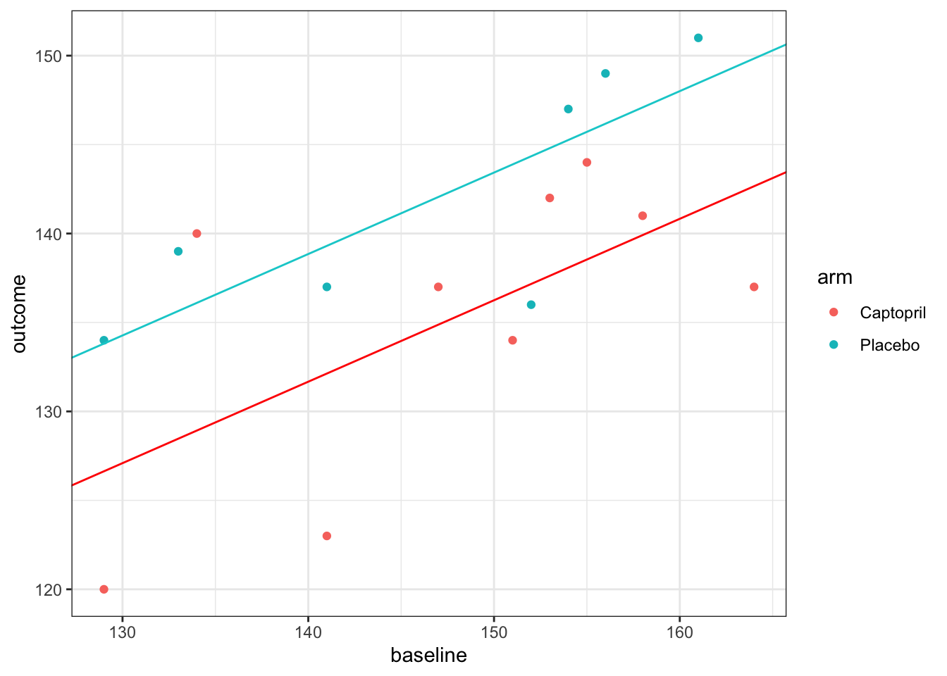
\[ \text{arm}_i = \begin{cases} 0 & \text{ if participant }i\text{ is assigned Captopril}\\ 1 & \text{ if participant }i\text{ is assigned Placebo}. \end{cases} \] Therefore, for a patient assigned Placebo, a value of 7.18 is added, as well as the intercept and baseline term. This results in a model with two parallel fitted lines.
For our previous methods we have calculated a confidence interval for the treatment effect \(\tau\), and we will do that here too. The second column of the linear model summary (above) gives the standard errors of each estimated parameter, and we see that the standard error of \(\hat{\tau}\) is 2.96. Therefore, to construct a 95/% confidence interval for \(\hat{\tau}\), we use (to 2 decimal places)
\(7.18\; \pm\; t_{0.975;13}\times{2.96} = \left(0.78,\; 13.57\right).\)
The model has \(n-p=13\) degrees of freedom because there are \(n=16\) data points and we are estimating \(p=3\) parameters. Notice that unlike our previous confidence intervals, this doesn’t contain zero, and so our analysis has enabled us to conclude that there is a significant reduction in blood pressure with Captopril. You can also see this in that \(p=0.03079<0.05\). However, you can tell from the width of the interval (and the fact that \(p\) is still quite close to 0.05) that there is still a lot of uncertainty about \(\tau\).
The ‘Residual standard error’ term near the bottom of the linear model summary is the estimate of \(\hat{\sigma_\epsilon}\), so here we have \(\hat{\sigma_\epsilon}^2 = 5.869^2 = 34.44.\)
As with any fitted model, we should check the residuals.
resid_capt = resid(lm_capt)
df_hommel$resid= resid_capt

ggplot(data = df_hommel, aes(x=baseline, y=resid, col=arm)) +
  geom_point() +
  geom_hline(yintercept=0)+
  xlab("Baseline")+
  ylab("Residual")+theme_bw()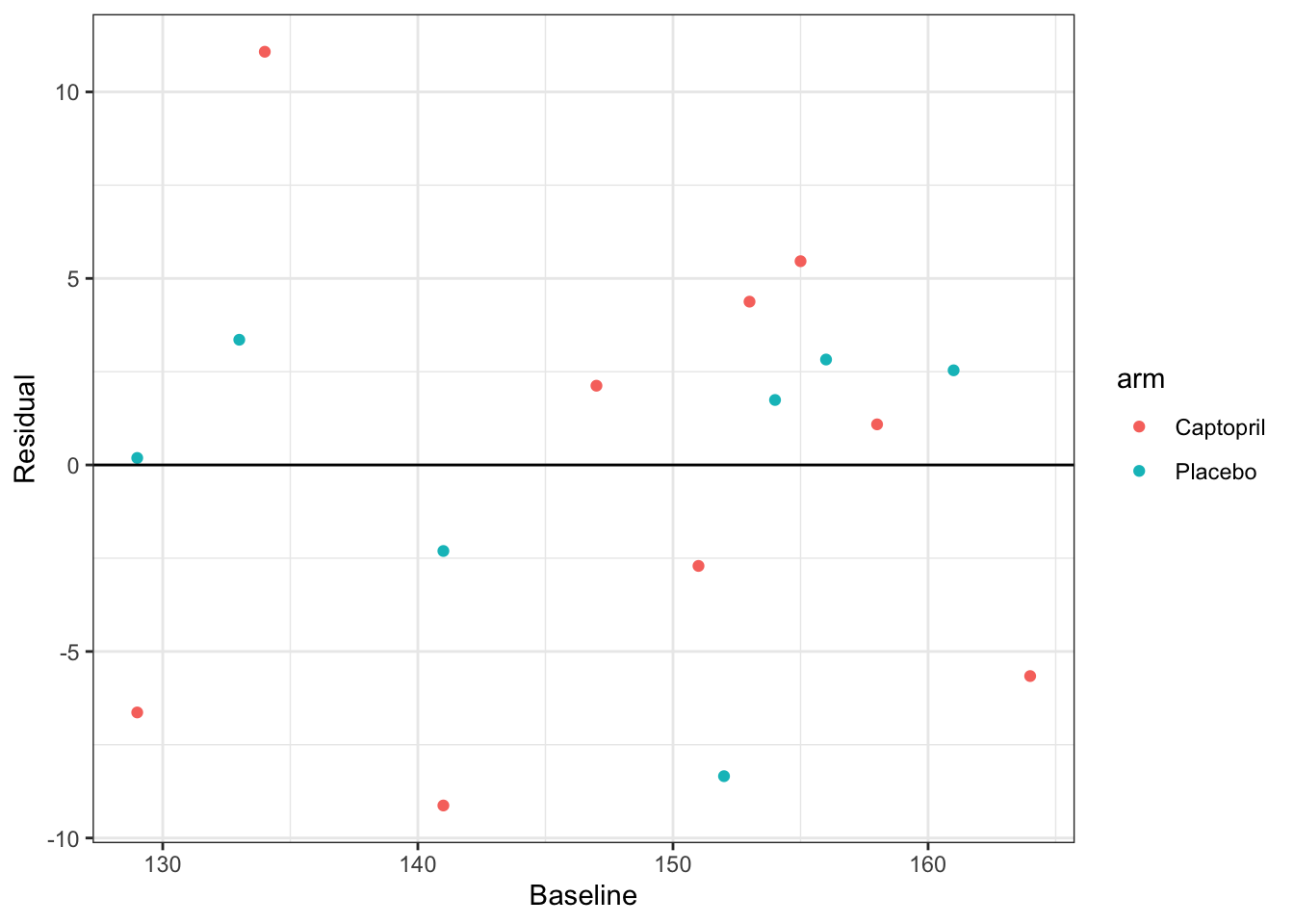
These look pretty good; there are no clear patterns and the distribution appears to be similar for each treatment group. Though, with such a small sample it’s difficult really to assess the fit of the model.
4.4 Some follow-up questions….
This might have raised a few questions, so we will address those now.
4.4.1 Didn’t we say that \(X_T - X_C\) was an unbiased estimator of \(\tau\)?
In Sections 4.1 and 4.2 we used both \(\bar{X}_T - \bar{X}_C\) and \(\left(\bar{X}_T - \bar{B}_T\right) - \left(\bar{X}_C - \bar{B}_C\right)\) as unbiased estimators of \(\tau\). Then, in Section 4.3.1 we showed that
\[ \begin{aligned} \operatorname{E}\left(\bar{X}_T - \bar{X}_C\mid{\bar{b}_T,\;\bar{b}_C}\right)& = \tau + \rho\left(\bar{b}_T - \bar{b}_C\right)\\ \operatorname{E}\left[\left(\bar{X}_T - \bar{b}_T\right) - \left(\bar{X}_C - \bar{b}_C\right)\mid{\bar{b}_T,\,\bar{b}_C}\right] &= \tau + \left(\rho-1\right)\left(\bar{b}_T - \bar{b}_C\right), \end{aligned} \] that is, neither of these quantities are unbiased estimators of \(\tau\) (except in very specific circumstances).
Is this a contradiction?
You’ll be relieved to hear (and may already have realised) that it isn’t; the first pair of equations are blind to the baseline values \(B_T\) and \(B_C\), and are using their statistical properties. Because of the randomisation procedure, a priori they can be treated the same. However, once we have observed values for the baseline, \(b_T\) and \(b_C\), they are very unlikely to be exactly the same. They are also (along with all other baseline measurements, often things like age, sex, height etc.) definitely not affected by the trial, since they are taken before any placebo or treatment has been administered, and often even before allocation. However, conditioning on their observed values can reduce the variance of our estimate of \(\tau\), as we have seen.
In this sense, the observed baseline means \(\bar{b}_T\) and \(\bar{b}_C\) are known as ancillary statistics; they contain no direct information about the parameter we are interested in (in this case the treatment effect \(\tau\)), but our inferences can be improved by conditioning on the observed values of the ancillary statistics.
4.4.2 What if the lines shouldn’t be parallel? The unequal slopes model
In the analysis above, we have assumed that the coefficient \(\gamma\) of baseline is the same in both groups; we have fitted an equal slopes model. It isn’t obvious that this should be the case, and indeed we can test for it.
Allowing each group to have a different slope means including an interaction term between baseline and treatment group,
\[ x_i = \mu + \tau G_i+ \gamma b_i + \lambda b_i G_i + \epsilon_i . \] The term \(\lambda b_i G_i\) is 0 if participant \(i\) is in group \(C\) and \(\lambda b_i\) if participant \(i\) is in group \(T\). Therefore, for participants in group \(C\), the gradient is still \(\gamma\), but for participants in group \(T\) it is now \(\gamma + \lambda\). We can test whether this interaction term should be included (that is, whether we should fit an unequal slopes model) by including it in a model and analysing the results.
Example 4.8 Continuing once again with the Captopril dataset, we now fit the model
lm_capt_int = lm(outcome ~ arm + baseline + baseline:arm, data = df_hommel)
tbl_regression(lm_capt_int)| Characteristic | Beta | 95% CI1 | p-value |
|---|---|---|---|
| arm | |||
| Captopril | — | — | |
| Placebo | 8.7 | -80, 98 | 0.8 |
| baseline | 0.46 | 0.05, 0.87 | 0.031 |
| arm * baseline | |||
| Placebo * baseline | -0.01 | -0.61, 0.59 | >0.9 |
| 1 CI = Confidence Interval | |||
We see that the \(p\)-value for the coefficient \(\lambda\) (seen in the arm:baseline row) is not at all significant (0.97). Therefore we can be confident that there is no need to fit unequal slopes for this dataset. This fits with our earlier conclusion (from inspecting the residuals) that just including first order terms is fine.
4.4.3 Can we include any other baseline covariates?
In Section 4.2 when our estimated treatment effect was \(\hat\tau = \left(\bar{x}_T - \bar{b}_T\right) - \left(\bar{x}_C - \bar{b}_C\right)\), the only other variable we could take into account was the baseline measurement, because it is on the same scale as the outcome \(X\). However, in ANCOVA, our treatment effect is
\[ \hat\tau = \left(\bar{x}_T - \bar{x}_C\right) - \hat\gamma\left(\bar{b}_T - \bar{b}_C\right), \] and the inclusion of the coefficient \(\gamma\) means that we can include other covariates on different scales too. The key issue is that we can only include as covariates things that were already known before allocation (hence they are sometimes known as baseline covariates, not to be confused with ‘the baseline’, which would generally mean the same measurement as the primary outcome, but before treatment). This is because they cannot, at that point, have been affected by the treatment, or have had an influence on the post-trial outcome measurement. Indeed, as a rule, any variable that was used in the randomisation procedure (this particularly applies to minimisation and stratified sampling) should be included in the analysis.
Example 4.9 The data for this example is taken from Kassambara (2019). In this study, 60 patients take part in a trial investigating the effect of a new treatment and exercise on their stress score, after adjusting for age. There are two treatment levels (yes or no) and three exercise levels (low, moderate and high) and 10 participants for each combination of treatment and exercise levels. Because in ANCOVA we fit a coefficient to every covariate, we can include exercise (another factor variable) and age (a continuous variable) in this analysis.
Table 4.6 shows the mean and standard deviation of age for each combination of treatment and exercise level. If we were being picky / thorough, we might note that (perhaps unsurprisingly!) the mean and standard deviation of age are both lower in the high exercise groups. This might well affect our analysis, but we won’t go into this now.
| Treatment | Exercise | Mean age | SD age |
|---|---|---|---|
| yes | low | 61.7 | 4.691600 |
| yes | moderate | 59.6 | 2.590581 |
| yes | high | 57.0 | 2.211083 |
| no | low | 62.1 | 4.332051 |
| no | moderate | 61.4 | 5.947922 |
| no | high | 57.9 | 3.381321 |
Fitting a linear model, we see that treatment, high levels of exercise and age each have a significant effect on stress.
##
## Call:
## lm(formula = score ~ treatment + exercise + age, data = stress)
##
## Residuals:
##     Min      1Q  Median      3Q     Max
## -9.0261 -3.7497 -0.4285  3.0943 13.3696
##
## Coefficients:
##                  Estimate Std. Error t value Pr(>|t|)
## (Intercept)      55.72934   10.91888   5.104 4.27e-06 ***
## treatmentno       4.32529    1.37744   3.140  0.00272 **
## exercisemoderate  0.08735    1.69032   0.052  0.95897
## exercisehigh     -9.61841    1.84741  -5.206 2.96e-06 ***
## age               0.49811    0.17648   2.822  0.00662 **
## ---
## Signif. codes:  0 '***' 0.001 '**' 0.01 '*' 0.05 '.' 0.1 ' ' 1
##
## Residual standard error: 5.288 on 55 degrees of freedom
## Multiple R-squared:  0.6045, Adjusted R-squared:  0.5757
## F-statistic: 21.01 on 4 and 55 DF,  p-value: 1.473e-10
We can calculate the variance inflation factor for this model
##               GVIF Df GVIF^(1/(2*Df))
## treatment 1.017841  1        1.008881
## exercise  1.230692  2        1.053264
## age       1.248533  1        1.117378
and see that values are fairly close to one.
In particular, taking a high level of exercise reduced participants’ stress scores by around 9.6, and the treatment reduced stress scores by around 4.3. Participants’ stress scores increased slightly with age (just under half a point per year!).
We can plot the residuals (Figure 4.4) to check that the model is a reasonable fit
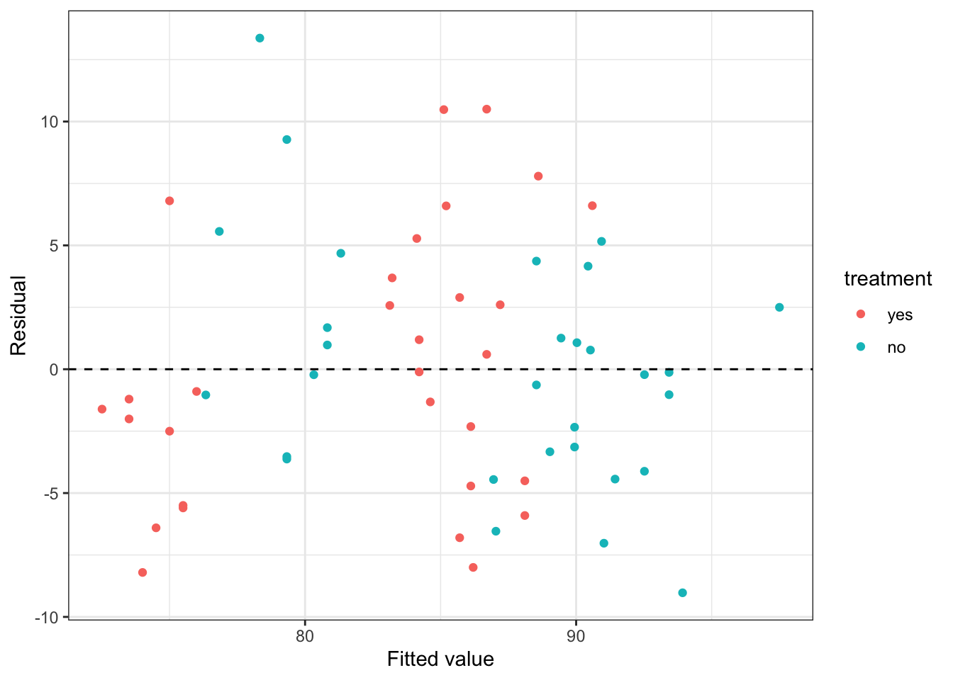
Figure 4.4: Residuals from the stress data model with only linear terms.
The first thing we notice is that the data are sort of ‘clumped’. This is common in factor models, especially where one or more factors is highly influential. Working from right to left (higher fitted stress score to lower), the highest clump (in blue) are those who do moderate or low levels of exercise and didn’t receive the treatment. The next clump (in red) are those who do moderate or low levels of exercise and did receive the treatment (their stress score is around 4.3 points lower, for the same age). The next clump, in blue, are those who do high levels of exercise and didn’t receive the treatment. Their scores are around 9.6 points lower than the low/moderate exercise groups who didn’t receive treatment. Finally, the lowest scoring group are those who do high levels of exercise and did receive the treatment. We see that some clumps aren’t really centred around zero, and this should raise alarm bells.
The data description says that the researchers want to test for the effect of ‘the intervention and exercise’ so it seems reasonable to include the interaction of these two terms:
##
## Call:
## lm(formula = score ~ treatment + exercise + age + treatment:exercise,
##     data = stress)
##
## Residuals:
##     Min      1Q  Median      3Q     Max
## -9.3250 -3.0192  0.2745  2.4650 10.6667
##
## Coefficients:
##                               Estimate Std. Error t value Pr(>|t|)
## (Intercept)                   56.79090   10.41383   5.453 1.32e-06 ***
## treatmentno                    1.52858    2.23026   0.685   0.4961
## exercisemoderate               0.01746    2.25662   0.008   0.9939
## exercisehigh                 -13.70331    2.36314  -5.799 3.78e-07 ***
## age                            0.50355    0.16684   3.018   0.0039 **
## treatmentno:exercisemoderate   0.15503    3.16129   0.049   0.9611
## treatmentno:exercisehigh       8.21822    3.15375   2.606   0.0119 *
## ---
## Signif. codes:  0 '***' 0.001 '**' 0.01 '*' 0.05 '.' 0.1 ' ' 1
##
## Residual standard error: 4.985 on 53 degrees of freedom
## Multiple R-squared:  0.6613, Adjusted R-squared:  0.623
## F-statistic: 17.25 on 6 and 53 DF,  p-value: 6.167e-11
Notice that now, the effect of the treatment on its own is not significant. Also notice that for both the linear exercise terms and the interactions between the exercise and treatment, the effects of moderate and low exercise are very similar.
This has somewhat improved the homogeneity of our residuals, as shown in Figure 4.5.
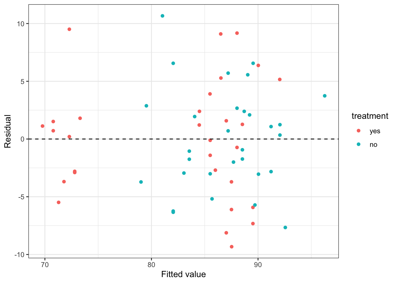
Figure 4.5: Residuals from the stress data model with the interaction between intervention and exercise included.
Combining the coefficients, someone who does a high level of exercise:
- is likely to reduce their stress score by around 13.7 if they receive the treatment
- is likely to reduce their stress score by around \(13.7 - 8.2 = 5.5\) if they don’t receive the treatment
Returning to our initial look at the dataset, the fact that age is a factor, and high levels of exercise are clearly very important should worry us slightly, since there are very few older people doing high levels of exercise. This may mean our model is inaccurate.
An important caution!
As you’ll have seen if you read Kendall (2003) (for formative assignment 1), we should have everything in place, including a statistical analysis plan, before the trial. We should already know which covariates we plan to include in our model, and how we are going to assess the fit. ‘Trawling’ for the best possible model by trying lots of different things (and inevitably settling on the one that leads to the most significant conclusion) is poor practice, and can increase the type I error rate (\(\alpha\)).
That said, it is crucial to check the model diagnostics, residual plots and so on, to make sure that the model is an appropriate one for the data. If there are problems (eg. if it appears that a particular covariate isn’t having a linear effect, or if there seems to be an interaction between two covariates) then you need to try different things until you get a good fit. This is different from p-fishing (described above), because you aren’t doing it to minimise the p-value. Indeed, the p-value might be higher for the model that best fits the data.
The way we’ve gone through analysis methods in this Section was to demonstrate and compare the different methods. Proceeding in the way we have, trying lots of different models, when analysing and writing up a trial would be very poor practice!
There’s another excellent episode of the JAMA Evidence podcast, with a focus on adjusting for covariates, that talks about this issue (you can find it here and linked from Ultra).
That draws to a close our work with continuous outcome variables. In the next lecture, we’ll start thinking about binary outcome variables.