8 Comparing survival curves
Really what we would like to be able to do is to compare two survival curves (showing, for example, the results from different treatments), so that we can say whether one is significantly different from the other. In most cases, this boils down to constructing a hypothesis test along the lines of
\[\begin{align*} H_0:&\text{ the treatments are the same}\\ H_1:&\text{ the treatments are different.} \end{align*}\]
There are various ways to do this, and we will look at some now.
8.1 Parametric: likelihood ratio test
For a parametric analysis, our null hypothesis that the two treatments are the same can be reduced to a test of whether the parameter(s) for each group are the same. We can do this using a likelihood ratio test. We’ve already calculated the log-likelihood for the exponential distribution in Section 7.2.2.1, and found the MLE.
\[\begin{align*} \ell\left(\lambda\right) & = m\log\lambda - \lambda\sum\limits_{i=1}^n t_i\\ \hat{\lambda} & = \frac{m}{\sum\limits_{i=1}^n t_i}. \end{align*}\]
Working with the exponential distribution, we can model the survival function as
\[S\left(t\right) = \begin{cases} e^{-\lambda_Ct}\; \text{ for participants in group C}\\ e^{-\lambda_Tt}\; \text{ for participants in group T} \end{cases} \] and the null hypothesis boils down to
\[H_0: \; \lambda_C = \lambda_T = \lambda. \] We can adapt the log-likelihood we found in Section 7.2.2.1 in light of the separate groups, and we find
\[\begin{equation} \ell\left(\lambda_C,\,\lambda_T\right) = m_C\log\lambda_C - \lambda_C\sum\limits_{i=1}^{n_C}t_{iC} + m_T\log\lambda_T - \lambda_T\sum\limits_{i=1}^{n_T}t_{iT} \tag{8.1} \end{equation}\]
and
\[\hat{\lambda}_X = \frac{m_X}{\sum\limits_{i=1}^{n_X}t_{iX}}\] where \(X=C\) or \(T\). In these equations \(m_X\) is the number of non-censored observations in group \(X\), \(n_X\) is the total number of participants in group \(X\) and \(t_{iX}\) is the time for participant \(i\) in group \(X\). To simplify notation, we will write
\[t^+_X = \sum\limits_{i=1}^{n_X}t_{iX},\] and \(t^+\) for the sum over both groups.
Substituting the MLEs into Equation (8.1) gives
\[\ell\left(\hat{\lambda}_C,\,\hat{\lambda}_T\right) = m_C\log\left(\frac{m_C}{t^+_C}\right) - m_C + m_T\log\left(\frac{m_T}{t^+_T}\right) - m_T \] and
\[\ell\left(\hat\lambda,\,\hat\lambda\right) = m\log\left(\frac{m}{t^+}\right) - m,\] where \(n,\,m\) are the corresponding totals over both groups.
We can therefore perform a maximum likelihood test by finding
\[\begin{align*} \lambda_{LR}& = -2\left[\ell\left(\hat{\lambda},\hat{\lambda}\right) - \ell\left(\hat{\lambda}_C,\hat{\lambda}_T\right)\right] \\ & = 2\left[\left(m_C\log\left(\frac{m_C}{t^+_C}\right) - m_C + m_T\log\left(\frac{m_T}{t^+_T}\right) - m_T \right) - \left(m\log\left(\frac{m}{t^+}\right)\right)\right]\\ & = 2\left(m_C\log\left(\frac{m_C}{t^+_C}\right) + m_T\log\left(\frac{m_T}{t^+_T}\right) - m\log\left(\frac{m}{t^+}\right)\right) \end{align*}\]
and referring this value to a \(\chi^2_1\) distribution.
We can also find a confidence interval for the difference between \(\lambda_T\) and \(\lambda_C\), by using the asymptotic variances of the MLEs, which are \(\frac{\lambda_C^2}{m_C}\) and \(\frac{\lambda_T^2}{m_T}\). Therefore, the limits of a \(100\left(1-\alpha\right)\)% CI for \(\lambda_T - \lambda_C\) are given by
\[ \frac{m_T}{t^+_T} - \frac{m_C}{t^+_C} \pm z_{\alpha/2}\sqrt{\frac{m_T}{\left(t^+_T\right)^2} + \frac{m_C}{\left(t^+_C\right)^2}}.\]
Example 8.1 In this example we’ll conduct a likelihood ratio test for each of the datasets in Example 7.1. For each dataset, the quantities we need are:
- \(m_C,\,m_T\): the number of complete observations in each group
- \(t^+_C,\,t^+_T\) the sum of all observation times (including censored times) in each group
Note that \(m=m_C + m_T\) and \(t^+ = t^+_C + t^+_T\).
For the ovarian data we have
mC_ov = sum((ovarian$fustat==1)&(ovarian$rx==1))
mT_ov = sum((ovarian$fustat==1)&(ovarian$rx==2))
tsum_ov_C = sum(ovarian$futime[ovarian$rx==1])
tsum_ov_T = sum(ovarian$futime[ovarian$rx==2])
m_ov = mT_ov + mC_ov
tsum_ov = tsum_ov_C + tsum_ov_T

## Can now plug these into LR test stat
LRstat_ov =  2*(mC_ov*log(mC_ov/tsum_ov_C) + mT_ov*log(mT_ov/tsum_ov_T) - m_ov*log(m_ov/tsum_ov))
LRstat_ov
## [1] 1.114895We can find the p-value of this test by
## [1] 0.2910204and we find that it isn’t significant. A 95% confidence interval for the difference is given by
## [1] -0.0013927697 0.0004392714For the Myeloid data we can do the same thing
mC_my = sum((myeloid$death==1)&(myeloid$trt=="A"))
mT_my = sum((myeloid$death==1)&(myeloid$trt=="B"))
tsum_my_C = sum(myeloid$futime[myeloid$trt=="A"])
tsum_my_T = sum(myeloid$futime[myeloid$trt == "B"])
m_my = mT_my + mC_my
tsum_my = tsum_my_C + tsum_my_T

## Can now plug these into LR test stat
LRstat_my =  2*(mC_my*log(mC_my/tsum_my_C) + mT_my*log(mT_my/tsum_my_T) - m_my*log(m_my/tsum_my))
LRstat_my
## [1] 11.95293Again, we refer this to \(\chi^2_1\):
## [1] 0.0005456153This time we find that the difference is significant at even a very low level, and the 95% CI is given by
## [1] -3.028814e-04 -8.108237e-05Although the confidence around \(\hat\lambda_X\) is high (ie. small standard error of the estimate), because of the large amount of data, the fit appears to actually be rather poor (recall Figure 7.7), mainly because of the inflexibility of the exponential distribution.
One feature of the exponential model that is convenient is that the hazard function is constant. Comparisons between treatment groups in survival trials are often summarised by the hazard ratio: the ratio of the hazard functions for the two groups. In general this is a function of \(t\), but for two exponential hazard functions it is simply the ratio of the \(\lambda\) values.
We could also perform LR tests with the fitted Weibull distributions, but instead we will continue on through some more commonly used methods.
8.2 Non-parametric: the log-rank test
The log-rank test is performed by creating a series of tables, and combining the information to find a test statistic.
We work through each time \(t_j\) at which an event is observed (by which we mean a death or equivalent, not a censoring) in either of the groups.
For notation, we will say that at time \(t_j\),
- \(n_j\) patients are ‘at risk’ of the event
- \(d_j\) events are observed (often the ‘event’ is death, so we will sometimes say this)
For groups \(C\) and \(T\) we would therefore have a table representing the state of things at time \(t_j\), with this general form:
| Group | No. surviving | No. events | No. at risk |
|---|---|---|---|
| Treatment | \(n_{Tj}-d_{Tj}\) | \(d_{Tj}\) | \(n_{Tj}\) |
| Control | \(n_{Cj}-d_{Cj}\) | \(d_{Cj}\) | \(n_{Cj}\) |
| Total | \(n_j-d_j\) | \(d_j\) | \(n_j\) |
Under \(H_0\), we expect the deaths (or events) to be distributed proportionally between groups \(C\) and \(T\), and so the expected number of events in group \(X\) (\(C\) or \(T\)) at time \(t_j\) is
\[e_{Xj} = n_{Xj}\times{\frac{d_j}{n_j}}.\] This means that \(e_{Cj}+e_{Tj} = d_{Cj} + d_{Tj} = d_j\).
If we take the margins of the table (by which we mean \(n_j, \,d_j,\,n_{Cj}\) and \(n_{Tj}\)) as fixed, then \(d_{Cj}\) has a hypergeometric distribution.
Definition 8.1 The hypergeometric distribution is a discrete probability distribution describing the probability of \(k\) successes in \(n\) draws (without replacement), taken from a finite population of size \(N\) that has exactly \(K\) objects with the desired feature. The probability mass function for a variable \(X\) following a hypergeometric function is
\[p\left(X=k\mid{K,N,n}\right) = \frac{{\binom{K}{k}}{\binom{N-K}{n-k}}}{{\binom{N}{n}}}. \] An example would be an urn containing 50 (\(N\)) balls, of which 16 (\(K\)) are green and the rest (34, \(N-K\)) are red. If we draw 10 (\(n\)) balls without replacement, \(X\) is the random variable whose outcome is \(k\), the number of green balls drawn.
In the notation of the definition, the mean is
\[\operatorname{E}\left(X\right)= n\frac{K}{N} \] and the variance is
\[\operatorname{var}\left(X\right) = n\frac{K}{N}\frac{N-K}{N}\frac{N-n}{N-1}.\]
In the notation of our table at time \(t_j\), we have
\[\begin{align*} \operatorname{E}\left(d_{Cj}\right) = e_{Cj} & = n_{Cj}\times{\frac{d_j}{n_j}}\\ \operatorname{var}\left(d_{Cj}\right) = v_{Cj} &= \frac{d_j n_{Cj}n_{Tj} \left(n_j-d_j\right)}{n_j^2\left(n_j-1\right)} \end{align*}\]
With the marginal totals fixed, the value of \(d_{Cj}\) fixes the other three elements of the table, so considering this one variable is enough.
Under \(H_0\), the numbers dying at successive times are independent, so
\[U = \sum\limits_{j}\left(d_{Cj}-e_{Cj}\right) \] will (asymptotically) have a normal distribution, with
\[U \sim {N}\left(0,\;\sum\limits_j v_{Cj}\right). \] We label \(V = \sum\limits_jv_{Cj}\), and in the log-rank test we refer \(\frac{U^2}{V}\) to \(\chi^2_1\).
A somewhat simpler, and more commonly used, version of the log-rank test uses the fact that under \(H_0\), the expected number of events (eg. deaths) in group \(X\) is \(E_X = \sum\limits_je_{Xj}\), and the observed number is \(O_X = \sum\limits_j d_{Xj}\). The standard \(\chi^2\) test formula can then be applied, and the test-statistic is
\[\frac{\left(O_C - E_C\right)^2}{E_C} + \frac{\left(O_T - E_T\right)^2}{E_T}.\]
It turns out that this test statistic is always smaller than \(\frac{U^2}{V}\), so this test is slightly more conservative (ie. it has a larger p-value).
Notice that for both of these test statistics, the actual difference between observed and expected is used, not the absolute difference. Therefore if the differences change in sign over time, the values are likely to cancel out (at least to some extent) and the log-rank test is not appropriate.
Example 8.2 Let’s now perform a log-rank test on our data from Example 8.1.
First, the ovarian cancer dataset. To do this, we can tabulate the key values at each time step.
| Time | n_Cj | d_Cj | e_Cj | n_Tj | d_Tj | e_Tj | n_j | d_j |
|---|---|---|---|---|---|---|---|---|
| 59 | 13 | 1 | 0.5000000 | 13 | 0 | 0.5000000 | 26 | 1 |
| 115 | 12 | 1 | 0.4800000 | 13 | 0 | 0.5200000 | 25 | 1 |
| 156 | 11 | 1 | 0.4583333 | 13 | 0 | 0.5416667 | 24 | 1 |
| 268 | 10 | 1 | 0.4347826 | 13 | 0 | 0.5652174 | 23 | 1 |
| 329 | 9 | 1 | 0.4090909 | 13 | 0 | 0.5909091 | 22 | 1 |
| 353 | 8 | 0 | 0.3809524 | 13 | 1 | 0.6190476 | 21 | 1 |
| 365 | 8 | 0 | 0.4000000 | 12 | 1 | 0.6000000 | 20 | 1 |
| 431 | 8 | 1 | 0.4705882 | 9 | 0 | 0.5294118 | 17 | 1 |
| 464 | 6 | 0 | 0.4000000 | 9 | 1 | 0.6000000 | 15 | 1 |
| 475 | 6 | 0 | 0.4285714 | 8 | 1 | 0.5714286 | 14 | 1 |
| 563 | 5 | 0 | 0.4166667 | 7 | 1 | 0.5833333 | 12 | 1 |
| 638 | 5 | 1 | 0.4545455 | 6 | 0 | 0.5454545 | 11 | 1 |
From this, we can find the \(v_{j}\) and the test statistic \(\frac{U^2}{V}\):
# Add up the differences
UC = sum(logrank_df$d_Cj - logrank_df$e_Cj)
vCj_vec = sapply(
  1:n_event,
  function(j){
    nCj = logrank_df$n_Cj[j]
    nTj = logrank_df$n_Tj[j]
    dj = logrank_df$d_j[j]
    nj = logrank_df$n_j[j]

    (nCj*nTj*dj*(nj-1))/((nj^2)*(nj-1))
})
VC = sum(vCj_vec)
cs_ov_stat = (UC^2)/VC
cs_ov_stat
## [1] 1.06274and refer it to \(\chi^2_1\)
## [1] 0.3025911For the simpler, more conservative, version of the log-rank test, we have
EC = sum(logrank_df$e_Cj)
ET = sum(logrank_df$e_Tj)
OC = sum(logrank_df$d_Cj)
OT = sum(logrank_df$d_Tj)

test_stat = ((EC-OC)^2)/EC + ((ET-OT)^2)/ET

test_stat
## [1] 1.057393and we can find the p-value by
## [1] 0.3038106As we expected, slightly larger, but not much different from the first version. These values are also pretty close to the results of our LR test in Example 8.1, where we had \(p=0.291\).
Since the Myeloid dataset is much bigger, we won’t go through the rigmarole of making the table, but will instead use an inbuilt R function from the survival package (more on this in practicals).
## Call:
## survdiff(formula = Surv(futime, death) ~ trt, data = myeloid,
##     rho = 0)
##
##         N Observed Expected (O-E)^2/E (O-E)^2/V
## trt=A 317      171      143      5.28      9.59
## trt=B 329      149      177      4.29      9.59
##
##  Chisq= 9.6  on 1 degrees of freedom, p= 0.002
This time the p-value is quite far from the one we found using the likelihood ratio test (p=0.00055), further supporting the view that the likelihood ratio test was not appropriate because of the poor fit of the exponential distribution.
8.3 Semi-parametric: the proportional hazards model
As with continuous and binary outcome variables, what we would really like to be able to do is to adjust our model for baseline covariates. It seems intuitively reasonable to suppose that factors like age, sex, disease status etc. might affect someone’s chances of survival (or whatever event we’re concerned with).
The conventional way to do this is using a proportional hazards model, where we assume that
\[h_T\left(t\right) = \psi h_C\left(t\right) \] for any \(t>0\) and for some constant \(\psi>0\). We call \(\psi\) the relative hazard or hazard ratio. If \(\psi<1\) then the hazard at time \(t\) under treatment \(T\) is smaller than under control \(C\). If \(\psi>1\) then the hazard at time \(t\) is greater in greater in group \(T\) than in group \(C\). The important point is that \(\psi\) doesn’t depend on \(t\). The hazard for a particular patient might be greater than for another, due to things like their age, disease history, treatment group and so on, but the extent of this difference doesn’t change over time.
We can adopt the concept of a baseline hazard function \(h_0\left(t\right)\), where for someone in group \(C\) (for now), their hazard at time \(t\) is \(h_0\left(t\right)\), and for someone in group \(T\) it is \(\psi h_0\left(t\right)\). Since we must have \(\psi>0\), it makes sense to set
\[\psi = e^{\beta},\] so that \(\beta = \log\psi\) and \(\psi>0\;\forall\beta\in\mathbb{R}\). Note that \(\beta>0 \iff \psi>1\).
We can now (re)-introduce our usual indicator variable \(G_i\), where
\[ G_i = \begin{cases} 0\text{ if participant }i\text{ is in group }C\\ 1\text{ if participant }i\text{ is in group }T \end{cases} \]
and model the hazard function for participant \(i\) as
\[h_i\left(t\right) = \exp\left[\tau G_i\right]h_0\left(t\right).\]
This is the proportional hazards model for the comparison of two groups. Now, the relative hazard is a function of the participant’s characteristics. Naturally, we can extend it to include other baseline covariates, as we have with linear models in ANCOVA, and with logistic regression.
8.3.1 General proportional hazards model
Extending the model to include baseline covariates \(X_1,\ldots,X_p\), we have
\[\psi\left(\mathbf{x}_i\right) = \exp\left(\tau G_i + \beta_1x_{1i} + \ldots + \beta_p x_{pi}\right) = \exp\left(\mathbf{x}_i^T \boldsymbol\beta\right),\] where we collect \(\tau\) into \(\boldsymbol\beta\) and \(G\) into \(\mathbf{x}\), and the hazard function for participant \(i\) is
\[h_i\left(t\right) = \psi\left(\mathbf{x}_i\right)h_0\left(t\right). \]
Now, our baseline hazard function \(h_0\left(t\right)\) is the hazard function for a participant in group \(C\) for whom all baseline coviariates are either zero (if continuous) or the reference level (if a factor variable). For factor covariates this makes sense, since all levels are realistic values, but for continuous variables zero is likely to be unrealistic (for example you’d never expect zero for age, weight, height, blood pressure etc.). So, if any continuous variables are present, the baseline will always need to be adjusted, but if all covariates are factors, it is likely that the baseline hazard function will be applicable for some set of participants.
The linear component \(\mathbf{x}_i^T\boldsymbol\beta\) is often called the risk score or prognostic index for participant \(i\).
The general form of the model is therefore
\[\begin{equation} h_i\left(t\right) = \exp\left[\mathbf{x}_i^T\boldsymbol\beta\right]h_0\left(t\right), \tag{8.2} \end{equation}\]
and we can rewrite it as
\[\log\left(\frac{h_1\left(t\right)}{h_0\left(t\right)}\right) = \mathbf{x}_i^T\boldsymbol\beta.\]
Notice that there is no constant in the linear term - if there was, it could just be absorbed into the baseline hazard function.
There are ways of fitting this model that rely on specifying the hazard function using parametric methods, but the method we will study (and the most widely used) is one developed by Cox (1972).
8.3.1.1 Interpreting the parameters in a proportional hazards model
Since our primary interest is in comparing the effect of some new treatment with that of the control, it is important that we understand what the coefficients mean, and in particular how they relate to the treatment effect. Let’s do that (as usual) by considering two participants who are identical in all baseline covariates, one in group C and one in group T. We have
\[\begin{align*} h^C_i\left(t\right) & = \exp\left(\beta_1x_{1i} + \ldots + \beta_p x_{pi}\right)h_0\left(t\right) & \text{ in group C}\\ h^T_i\left(t\right) & = \exp\left(\tau + \beta_1x_{1i} + \ldots + \beta_p x_{pi}\right)h_0\left(t\right) & \text{ in group T.} \end{align*}\]
From this we can find the hazard ratio at time \(t\) for the two treatments to be
\[\frac{h^T_i\left(t\right)}{h^C_i\left(t\right)} = \exp{\left(\tau\right)} \] and \(\tau\) is the log of the hazard ratio for the two treatments, adjusting for the other covariates. A value of \(\tau=0\) implies a hazard ratio of one, and of no evidence of difference between the treatments.
8.3.2 Cox regression
The beauty of Cox regression is that it avoids specifying a form for \(h_0\left(t\right)\) altogether.
To fit the model in Equation (8.2) we must estimate the coefficients \(\boldsymbol\beta = \left(\tau,\,\beta_1,\ldots,\beta_p\right)^T\). It also appears as though we should estimate the baseline hazard \(h_0\left(t\right)\) somehow too, but the great advance made by Cox was to develop a method where this isn’t necessary. We don’t need to estimate \(h_0\left(t\right)\) to make inferences about the hazard ratio
\[\frac{h_i\left(t\right)}{h_0\left(t\right)}.\] We will estimate the coefficients \(\boldsymbol\beta\) using maximum likelihood, and so we’ll need to specify a likelihood function for the \(\boldsymbol\beta\), which will be a function of \(\mathbf{x}^T\boldsymbol\beta\) and our observed data, the survival times \(t_i\).
Suppose we have data for \(n\) participants, and that these include \(m\) complete observations (often referred to as deaths) and \(n-m\) right-censored survival times. Suppose also that all the complete observation times are distinct. Since time itself is continuous, this is always technically true, but in data the time will be rounded and so there may be multiple observations at one time.
We can order these \(m\) event times
\[t_{(1)}< t_{(2)} < \ldots < t_{(m)},\] such that \(t_{(j)}\) is the time of the \(j^{\text{th}}\) event to be observed.
At time \(t_{(j)}\), there will be some number of individuals who are ‘at risk’ of the event, because either their observation time or their censored survival time is greater than \(t_{(j)}\). The set of these individuals is the risk set, denoted \(R\left(t_{(j)}\right)\).
Cox (1972) shows that the relevant likelihood function for the proportional hazards model in Equation (8.2) is
\[\begin{equation} L\left(\boldsymbol\beta\right) = \prod\limits_{j=1}^m\frac{\exp\left[\mathbf{x}_{(j)}^T\boldsymbol\beta\right]}{\sum\limits_{l\in R\left(t_{(j)}\right)}{\exp\left[\mathbf{x}_l^T\boldsymbol\beta\right]}} \tag{8.3} \end{equation}\]
where \(\mathbf{x}_{(j)}\) is the vector of covariates for the individual who dies (or equivalent) at time \(t_{(j)}\). Notice that the product is over only those individuals with complete observations, but individuals with censored data do contribute to the sum in the denominator.
The numerator of the fraction inside the product in Equation (8.3) is the relative hazard for the person who actually did die at time \(t_{(j)}\). The denominator is the sum of the relative hazards for all those who possibly could have died at time \(t_{(j)}\) (the risk set \(R\left(t_{(j)}\right)\)). Thus, in very loose terms, maximizing the likelihood means finding values for \(\boldsymbol\beta\) that mean the people who did die were ‘the most likely’ to die at the time they did.
Notice that this is not a true likelihood, since it depends only on the ordering of the data (the observation and censoring times) and not the data itself. This makes it a partial likelihood. The argument given to justify this is that because the baseline hazard \(h_0\left(t\right)\) has an arbitrary form, it’s possible that except for at these observed times, \(h_0\left(t\right)=0\), and therefore \(h_i\left(t\right)=0\). This means the intervals between successive observations convey no information about the effect of the covariates on hazard, and therefore about the \(\boldsymbol\beta\) parameters.
If you want to know more detail about how this likelihood was derived, you can find in in Section 3.3 of Collett (2003b), or in Cox’s original paper (Cox (1972)).
Moving on, if we set
\[ \delta_i = \begin{cases} 0\;\;\text{ if individual }i\text{ is censored}\\ 1\;\;\text{ if individual }i\text{ is observed} \end{cases} \] then we can write Equation (8.3) as
\[L\left(\boldsymbol\beta\mid{\text{data}}\right) = \prod\limits_{i=1}^n\left(\frac{\exp\left[\mathbf{x}_i^T\boldsymbol\beta\right]}{\sum\limits_{l\in R\left(t_i\right)}{\exp\left[\mathbf{x}_l^T\boldsymbol\beta\right]}}\right)^{\delta_i},\] where \(R\left(t_i\right)\) is the risk set at time \(t_i\).
From this we can find the log-likelihood
\[\ell\left(\boldsymbol\beta\mid{\text{data}}\right) = \sum\limits_{i=1}^n \delta_i\left[\mathbf{x}_i^T\boldsymbol\beta - \log\sum\limits_{l\in R\left(t_i\right)}\exp\left(\mathbf{x}_l^T\boldsymbol\beta\right)\right].\] The MLE \(\hat{\boldsymbol\beta}\) is found using numerical methods (often Newton-Raphson, which you’ll have seen if you did Numerical Analysis II).
How can we tell if a proportional hazards model is appropriate?
We can’t easily visualise the hazard function for a dataset, and instead would plot the survival curve. So can we tell if the proportional hazards assumption is met by looking at the survival curve?
It turns out that if two hazard functions are proportional, their survival functions won’t cross one another, as we will show now.
Suppose \(h_C\left(t\right)\) is the hazard at time \(t\) for an individual in group \(C\), and \(h_T\left(t\right)\) is the hazard for that same individual in group \(T\). If the two hazards are proportional then we have (as before)
\[h_T\left(t\right) = \psi h_C\left(t\right) \] for some constant \(\psi\).
Recall from Section 7.2 that
\[h\left(t\right) = \frac{f\left(t\right)}{S\left(t\right)},\] where \(S\left(t\right)\) is the survival function and \(f\left(t\right)\) is the probability density of \(T\). We can therefore write
\[h\left(t\right) = -\frac{d}{dt}\left[\log\left(S\left(t\right)\right)\right]\] and rearrange this to
\[\begin{equation} S\left(t\right) = \exp \left(-H\left(t\right)\right) \tag{8.4} \end{equation}\]
where \[H\left(t\right) = \int\limits_0^t h\left(u\right) du.\]
Therefore for our two hazard functions, we have
\[\exp\left\lbrace - \int\limits_0^t h_T\left(u\right)du \right\rbrace =\exp\left\lbrace -\int\limits_0^t\psi h_C\left(u\right) du \right\rbrace \] From Equation (8.4) we see that therefore
\[S_T\left(t\right) = \left[S_C\left(t\right)\right]^\psi.\] Since the survival function is always between 0 and 1, we can see that the value of \(\psi\) determines whether \(S_C\left(t\right)<S_T\left(t\right)\) (if \(0<\psi<1\)) or \(S_C\left(t\right)>S_T\left(t\right)\) (if \(\psi>1\)). The important thing is that the survival curves will not cross. This is an informal conclusion, and lines not crossing is a necessary condition but not a sufficient one.
This property can be helpful in working out what model to fit. For example, it may sometimes be that the survival curves don’t cross when a particular [influential] covariate is factored out, but do when it isn’t.
Example 8.3 First of all, we can use Cox regression adjusted only for the Group (or treatment arm) of the participants.
For the ovarian dataset
## Call:
## coxph(formula = Surv(futime, fustat) ~ rx, data = ovarian)
##
##       coef exp(coef) se(coef)      z    p
## rx -0.5964    0.5508   0.5870 -1.016 0.31
##
## Likelihood ratio test=1.05  on 1 df, p=0.3052
## n= 26, number of events= 12
and for the myeloid1 dataset
## Call:
## coxph(formula = Surv(futime, death) ~ trt, data = myeloid)
##
##         coef exp(coef) se(coef)      z       p
## trtB -0.3457    0.7077   0.1122 -3.081 0.00206
##
## Likelihood ratio test=9.52  on 1 df, p=0.002029
## n= 646, number of events= 320
We see that for both results, our p-values are close to what we have found with the log rank test.
For the ovarian dataset there is no evidence of a significant difference (likely due to the small sample size).
For the myeloid data we find that there is evidence of a difference - we can use the coefficient estimate and standard error to construct a 95% confidence interval for the log hazard ratio of
\[ -0.346 \pm 1.96 \times 0.112 = \left(-0.566,\, -0.126\right) \]
and therefore for the hazard ratio itself of
\[\left(0.568,\, 0.881\right). \] We see that there is strong evidence that the intervention reduces the hazard.
We can also account for more baseline covariates. For the ovarian data we can include age and resid.ds (whether residual disease is present):
## Call:
## coxph(formula = Surv(futime, fustat) ~ rx + age + resid.ds, data = ovarian)
##
##             coef exp(coef) se(coef)      z       p
## rx       -0.8489    0.4279   0.6392 -1.328 0.18416
## age       0.1285    1.1372   0.0473  2.718 0.00657
## resid.ds  0.6964    2.0065   0.7585  0.918 0.35858
##
## Likelihood ratio test=16.77  on 3 df, p=0.0007889
## n= 26, number of events= 12
What this shows is that the most significant factor by far is the particpant’s age, with the hazard function increasing as age increases. The coefficient for treatment group (rx) has increased in magnitude and the p-value has decreased now that age is being adjusted for (although it is still not significant).
We can do the same for the myeloid data:
## Call:
## coxph(formula = Surv(futime, death) ~ trt + sex, data = myeloid)
##
##         coef exp(coef) se(coef)      z       p
## trtB -0.3582    0.6989   0.1129 -3.174 0.00151
## sexm  0.1150    1.1219   0.1128  1.020 0.30782
##
## Likelihood ratio test=10.56  on 2 df, p=0.005093
## n= 646, number of events= 320
We see that the only covariate we have, sex has very little effect, and that our confidence interval for the treatment effect will not have changed much at all.
8.3.3 Diagnostics for Cox regression
Having fit a Cox proportional hazards model, it’s important to check that it is an appropriate fit to the data. We’ve seen already that the survival curves mustn’t cross, but there are other more sophisticated methods we can use to assess the model.
It is important to examine the proportional hazards assumption for every covariate we include in the model (including the group / arm variable), and how we do this depends on whether the covariate is continuous or categorical.
8.3.3.1 Continuous variables
Schoenfeld (1982) derived partial residuals, known as Schoenfeld residuals, that can be used to assess whether the proportional hazards assumption is appropriate for a continuous variable.
We can think of \(X_i = \left(X_{i1},\ldots,X_{ip}\right)'\), the set of covariates for a participant who experiences the event at time \(t_i\), as a random variable. Schoenfeld (1982) showed that
\[E\left(X_{ij}\mid{R_i}\right) = \frac{\sum\limits_{k\in{R_i}}X_{kj}\exp\left(\beta'X_k\right)}{\sum\limits_{k\in{R_i}}\exp\left(\beta'X_k\right)}, \] where \(R_i\) are the indices of those at risk at time \(t_i\). You can think of this as the average of the \(X_{\cdot j}\) values of those at risk as time \(t_i\), weighted by their relative hazard. We can write
\[ \hat{E}\left(X_{ij}\mid R_i\right)\] to denote this quantity with the MLE \(\hat\beta\) substituted for \(\beta\).
The partial residual at time \(t_i\) is therefore the vector
\[\hat{r} = \left(\hat{r}_{i1},\ldots,\hat{r}_{ip}\right), \]
where
\[\hat{r}_{ik} = X_{ik} - \hat{E}\left(X_{ik}\mid{R_i}\right). \] If we plot the Schoenfeld residuals against time, we should see a random scatter around zero (the kind of plot we look for when assessing residuals against fitted values of a linear regression model).
Grambsch and Therneau (1994) proposed a statistical test using the Schoenfeld residuals, in which the null hypothesis is that the proportional hazards assumption holds. This can be implemented by the function cox.zph in the survival package.
Example 8.4 The ovarian data contains the continuous variable age, and so we can test the assumption of proportional hazards in relation to age using Schoenfeld residuals.
##          chisq df    p
## rx       0.631  1 0.43
## age      0.210  1 0.65
## resid.ds 1.120  1 0.29
## GLOBAL   1.958  3 0.58
We see from the age line that the data are consistent with the proportional hazards assumption.
The object created by cox.zph also contains the Schoenfeld residuals themselves, and so we can plot them:

Because there is so little data it’s hard to conclude anything, and indeed our lack of significance in the test may be due to small sample size rather than excellent model fit.
8.3.3.2 Categorical variables
Recall from Equation (8.4) that
\[S\left(t\right) = \exp\left(-H\left(t\right)\right), \] where \(H\left(t\right)\) is the cumulative hazard function
\[ H\left(t\right) = \int\limits_{0}^t h\left(u\right) du. \]
From this we find that
\[ \log \left(S\left(t\right)\right) = -H\left(t\right).\]
If we have two groups \(A\) and \(B\) for which the proportional hazards assumption is satisfied, then for some constant \(\psi\)
\[H_A\left(t\right) = \psi H_B\left(t\right). \] We can combine these two equations to find
\[\begin{align*} \log\left[-\log\left(S_A\left(t\right)\right)\right] = \log\left(H_A\left(t\right)\right) & = \log\psi + \log\left(H_B\left(t\right)\right)\\ & = \log\psi + \log\left[-\log\left(S_B\left(t\right)\right)\right]. \end{align*}\]
Under the Cox Regression model, \(\log\left(H\left(t\right)\right)\) is linear in the covariates, and so we will have [roughly] parallel lines. We can plot this in R using ggsurvplot and setting fun="cloglog".
Example 8.5 First we’ll check the ovarian dataset, split by treatment group (Figure 8.1).
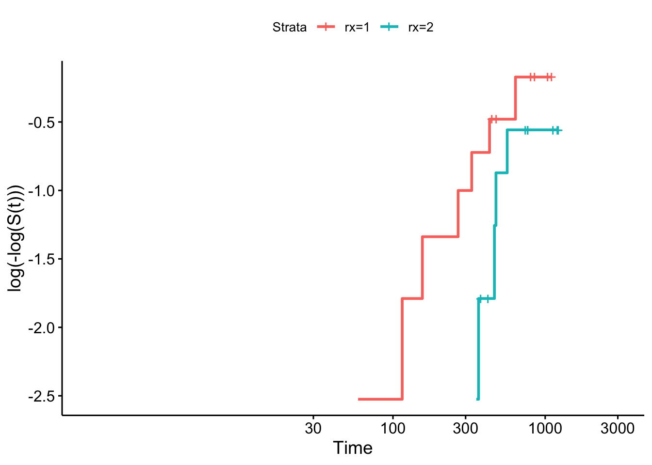
Figure 8.1: Log-log plot for ovarian data by treatment group.
As before, there isn’t really enough data to tell whether the assumption is violated.
We can do the same for the myeloid data, as in Figures 8.2 and 8.3.
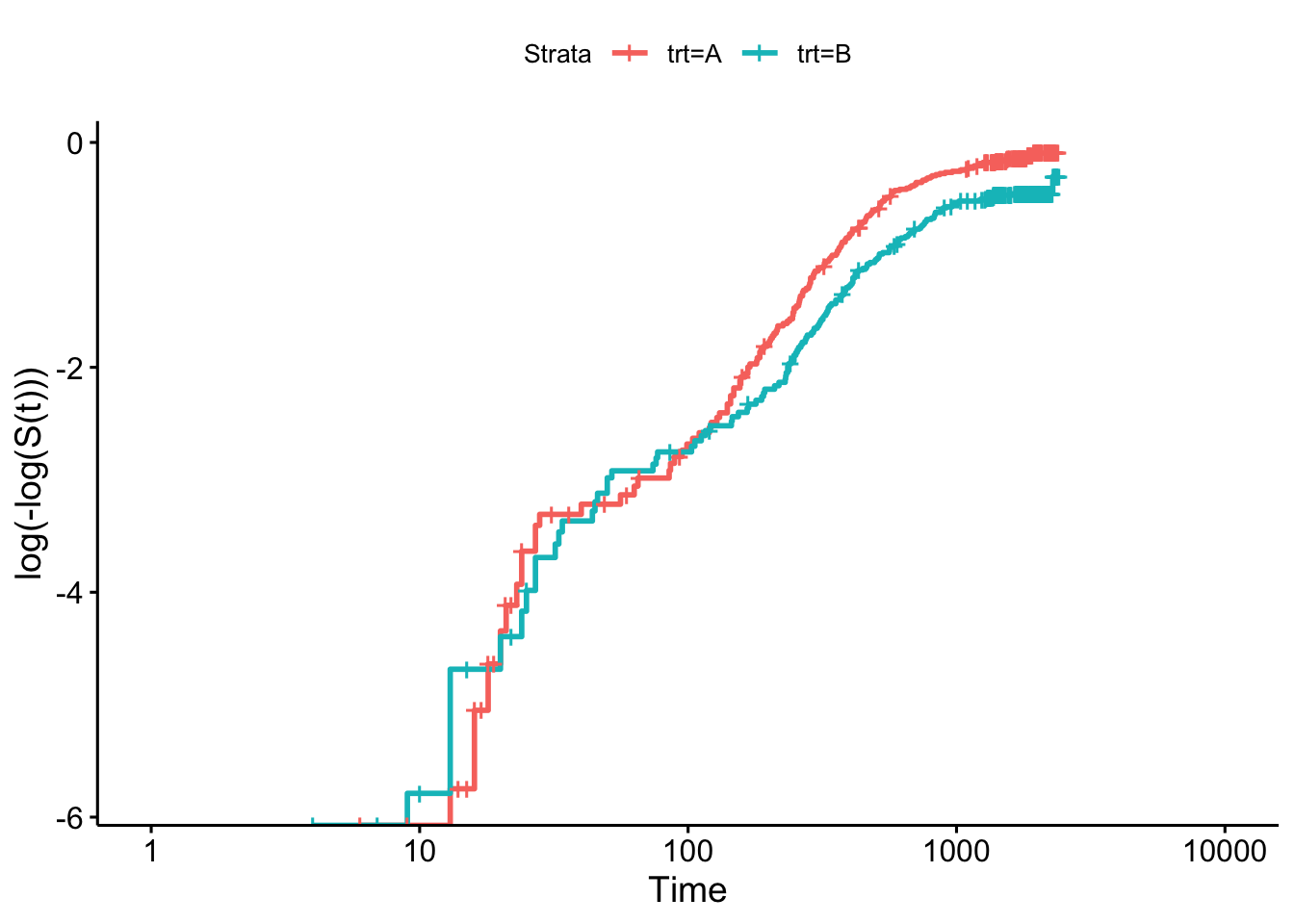
Figure 8.2: Log-log plot for myeloid data by treatment group.
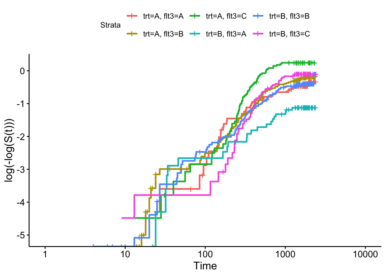
Figure 8.3: Log-log plot for myeloid data by treatment group.
To explore these diagnostic checks further we will introduce the veteran dataset, which focuses on a trial for lung cancer patients. The treatment variable is trt and there are a mixture of continuous and categorical covariates. We will include celltype, a categorical variable with four levels and karno, a score from 0 to 100 (which we will treat as continuous).
Firstly we can check the proportional hazards assumption for the categorical covariates, in Figure 8.4.
sf_vet = survfit(Surv(time, status) ~ trt+celltype, data=veteran)
ggsurvplot(sf_vet, fun = "cloglog")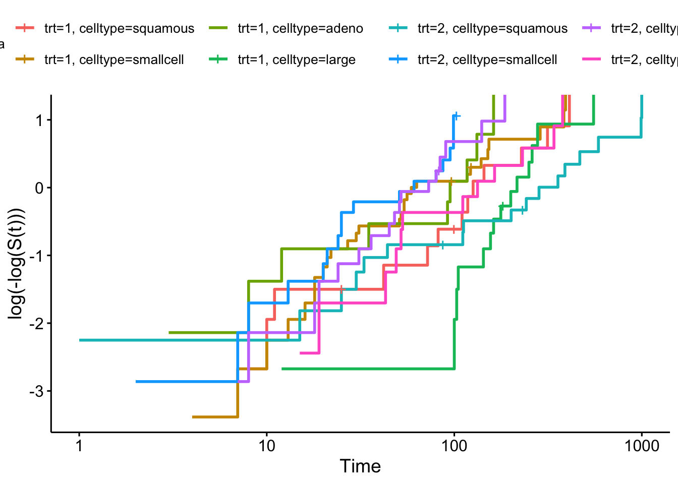
Figure 8.4: Log-log plot for veteran data split by treatment group and cell type
Next we can fit a Cox proportional hazards model
## Call:
## coxph(formula = Surv(time, status) ~ trt + celltype + karno,
##     data = veteran)
##
##   n= 137, number of events= 128
##
##                        coef exp(coef)  se(coef)      z Pr(>|z|)
## trt                0.261744  1.299194  0.200923  1.303  0.19267
## celltypesmallcell  0.824980  2.281836  0.268911  3.068  0.00216 **
## celltypeadeno      1.153994  3.170833  0.295038  3.911 9.18e-05 ***
## celltypelarge      0.394625  1.483828  0.282243  1.398  0.16206
## karno             -0.031271  0.969213  0.005165 -6.054 1.41e-09 ***
## ---
## Signif. codes:  0 '***' 0.001 '**' 0.01 '*' 0.05 '.' 0.1 ' ' 1
##
##                   exp(coef) exp(-coef) lower .95 upper .95
## trt                  1.2992     0.7697    0.8763    1.9262
## celltypesmallcell    2.2818     0.4382    1.3471    3.8653
## celltypeadeno        3.1708     0.3154    1.7784    5.6534
## celltypelarge        1.4838     0.6739    0.8534    2.5801
## karno                0.9692     1.0318    0.9595    0.9791
##
## Concordance= 0.737  (se = 0.022 )
## Likelihood ratio test= 61.07  on 5 df,   p=7e-12
## Wald test            = 63.41  on 5 df,   p=2e-12
## Score (logrank) test = 66.55  on 5 df,   p=5e-13
and check the Schoenfeld residuals for karno, as in Figure 8.5.

Figure 8.5: Schoenfeld residuals for Cox regression model fit to veteran data, for covariate ‘karno’
Although these look quite evenly spread, they are mostly negative, and it appears there is a slight trend with time. Indeed the p-value shows a significant deviation from proportional hazards.