10 Random effects for individuals
In the last lecture we introduced the mixed effects model as a way to combine fixed effects (the kind we’re used to, like sex, disease status etc.) and random effects. For cluster randomized trials this was useful because we could account for the intracluster correlation, where participants within the same school / GP surgery / other cluster are likely to be more similar to one another than to participants within another group.
In this lecture, we’ll think about a couple of examples where the individual is the random effect.
10.1 Crossover trials
In the trials we’ve thought about so far, each patient has been subject to one, and only one, treatment. Often this is necessary, because the end goal is something relatively final, like a disease being cured, or the circumstance is a one-off, like medication to prevent complications of surgery. By doing things this way, we lose the opportunity to make direct comparisons; we assume that all participants are randomly drawn from some population, and make efforts to ensure the trial is balanced in terms of their characteristics, but we can’t truly compare like-for-like.
Crossover trials, also known as AB or AB/BA trials, involve giving each participant both treatments in sequence. These are generally used in contexts where the goal is ongoing management of a condition, for example asthma or diabetes. If we give each participant each of the different treatments in sequence, then we can make a more precise comparison, since we are comparing the outcomes under the different treatments on the same patient. You can find more detail of this type of trial in Armitage and Hills (1982).
10.1.1 The AB/BA design
If we gave all patients treatment A first (say for one month) and then treatment B (for the next), then we would be inviting bias and ambiguity into the trial
- It may be that whichever treatment comes second appears to perform better, for example as patients get used to measurements being taken (it is common for the first few blood pressure measurements in a series to be higher)
- If there is some external trend or pattern, this will manifest itself as an effect of the change in treatments.
Therefore in a crossover trial with two treatments there are two groups, who receive the treatments in different orders:
| Group | Period 1 | Period 2 |
|---|---|---|
| Group 1 | A | B |
| Group 2 | B | A |
Therefore if there is a temporal effect it won’t be ascribed to either of the treatments.
10.1.2 Analysis of the AB/BA design
There are a few things our analysis needs to account for:
- Measurements for the same participant need to be treated as such, in some way
- The possibility of systematic differences between treatment periods needs to be allowed for
In the model we describe, we assume there are \(n_1\) participants in group 1, and \(n_2\) in group 2. We will also assume that the outcome is normally distributed. In the treatment of ongoing conditions, this is generally the case.
We will start by thinking about the outcome for particular individuals. We’ll assume that one outcome measurement is taken per patient per trial period. So the outcome for participant \(i\) \((i = 1,\ldots,n_1)\) from group 1 is modelled by
\[\begin{align*} x_{i1} & = \mu + \pi_1 + \tau_A + \xi_i + \epsilon_{i1} \text{ in trial period 1}\\ x_{i2} & = \mu + \pi_2 + \tau_B + \xi_i + \epsilon_{i2} \text{ in trial period 2.} \end{align*}\]
In this model
- \(\pi_j\;\;(j=1,2)\) is the systematic effect of period \(j\)
- \(\tau_A,\,\tau_B\) are the systematic effects of treatments A and B
- \(\mu\) is a general mean
- \(\xi_i\) represents the tendency for the outcome of participant \(i\) to be generally higher or lower than the mean
- \(\epsilon_{i1},\,\epsilon_{i2}\) are independent \(N\left(0,\,\sigma_{\epsilon}^2\right)\) error terms.
Notice that the first three bullet points describe fixed effects, and the fourth \((\xi_i)\) is a random effect. We can assume that \(\xi_i \sim N\left(0,\,\sigma_B^2\right)\). Notice that \(\xi_i\) appears in the outcome model for participant \(i\) for both trial periods.
We can us the same logic to model the outcome for participant \(i\) \(\left(i=n_1+1,\,\ldots,\,n_1+n_2\right)\) in group 2
\[\begin{align*} x_{i1} & = \mu + \pi_1 + \tau_B + \xi_i + \epsilon_{i1} \text{ in trial period 1}\\ x_{i2} & = \mu + \pi_2 + \tau_A + \xi_i + \epsilon_{i2} \text{ in trial period 2.} \end{align*}\]
Because we have been able to treat each participant with both treatments (A and B), we have effectively bundled all the participant specific covariates, along with individual variation we can’t really account for, into \(\xi_i\).
We can remove \(\xi_i\) from from the analysis by finding the differences for each patient
\[\begin{align*} d_i & = x_{i1} - x_{i2} = \pi + \tau + \eta_i& \text{ for } i=1,\,\ldots,\,n_1\\ d_i & = x_{i1} - x_{i2} = \pi - \tau + \eta_i& \text{ for } i=n_1+1,\,\ldots,\,n_1+n_2, \end{align*}\]
where
- \(\pi=\pi_1 - \pi_2\) measures the difference between treatment periods
- \(\tau = \tau_A - \tau_B\) is the treatment effect we are interested in
- \(\eta_i = \epsilon_{i1} - \epsilon_{i2}\) is another random error, with mean 0 and variance \(\sigma^2=2\sigma^2_{\epsilon}\)
We can take expected values of the differences, and find
\[\begin{align*} \operatorname{E}\left(d\right) & = \pi+\tau & \text{ in group 1}\\ \operatorname{E}\left(d\right) & = \pi-\tau & \text{ in group 2} \end{align*}\]
If there is no treatment effect, ie. \(\tau=0\), then we expect the means to be approximately equal.
This means we can test the null hypothesis that \(\tau=0\) with a two-sample \(t\)-test, to compare the two sets of within patient differences. Note, this is not a paired t-test: we are comparing the differences for the \(n_1\) participants in group 1 with the differences for the \(n_2\) participants in group 2.
An estimate of the treatment effect can be found using \[\frac{1}{2}\left(\bar{d}_1 - \bar{d}_2\right),\] where \(\bar{d}_k\) is the mean difference in group \(k\). We can therefore find a confidence interval by halving the limits of the usual confidence interval for the difference in two means.
Another important point to note is that since we have eliminated the individual participant random effect \(\xi_i\) from the analysis, the precision of the result depends only on \(\sigma^2_{\epsilon}\), and not on the between-individual variance \(\sigma^2_B\). This is especially good news in a scenario in which the measurement varies much more between individuals than within individuals. Intuitively this makes sense: it is best to use a patient as his or her own control.
Example 10.1 For children with nocturnal enuresis (bed-wetting) a drug is available to potentially alleviate the problem, and in this trial the drug is to be compared with a placebo, and the treatment period is two weeks. Children in group A are given the drug first, followed by the placebo. Children in group B are given the placebo first, followed by the drug. The primary outcome variable is the number of dry nights out of the 14 night of each treatment period. The data are shown in Table 10.1.
|
|
We can use this information to find the mean difference for each group
## [1] 2.823529## [1] -1.25Immediately we can see that these back up the notion that the drug is effective (remember the difference for group A is drug minus placebo, the difference for group B is placebo minus drug), and that the number of dry nights tends to be more while taking the drug.
To test the hypothesis more carefully we use a t-test.
##
##  Two Sample t-test
##
## data:  dfA$Diff and dfB$Diff
## t = 3.2925, df = 27, p-value = 0.002773
## alternative hypothesis: true difference in means is not equal to 0
## 95 percent confidence interval:
##  1.535005 6.612054
## sample estimates:
## mean of x mean of y
##  2.823529 -1.250000
We see that this backs up the hypothesis that the drug reduces nocturnal enuresis.
We could analyse the same dataset without taking into account the crossover design of the trial, simply by performing a t-test of all measurements on the drug against all measurement on the placebo
drug_meas = c(dfA$Period1,dfB$Period2)      # Measurements taken while on drug
placebo_meas = c(dfA$Period2, dfB$Period1)  # Measurements taken while on placebo
t.test(
  x=drug_meas, y=placebo_meas,
  paired=F, alternative="two.sided", var.equal=T)
##
## Two Sample t-test
##
## data: drug_meas and placebo_meas
## t = 2.253, df = 56, p-value = 0.0282
## alternative hypothesis: true difference in means is not equal to 0
## 95 percent confidence interval:
## 0.2408072 4.1040204
## sample estimates:
## mean of x mean of y
## 8.448276 6.275862We see that although the outcome is still significant at the \(\alpha=0.05\) level, the p-value is much larger, because the individual effects have not been taken into account.
10.2 Longitudinal data / repeated measurements
The second situation we will consider is where there are repeated measurements of the same participant: this is often called longitudinal data. So far we have considered only a baseline and final measurement of the outcome variable, but in practice it is common to measure the outcome at several points throughout the trial duration.
Clinicians may want to understand not just how the outcome is behaving at the end of the trial, but how it evolves over time. They may also want to understand the variation in the measurement over time; for example, it is reasonable to expect that a particular patient’s blood presssure or respiratory function won’t be exactly the same every day, even under the same treatment and general conditions.
In general we’ll say that we have two treatment groups, C (control) and T (treatment), containing \(n_C\) and \(n_T\) participants respectively. The \(i^{\text{th}}\) participant in group \(X\) is observed \(k_{Xi}\) times through the course of the trial. Generally (and we’ll certainly assume here) the measurements are planned to be at the same times.
Example 10.2 The first data set we’ll introduce is epilepsy, from the package HSAUR3. This trial (detailed in Thall and Vail (1990)) investigates the effect of an anti-epileptic drug called Progabide compared to a placebo (both groups were also receiving chemotherapy). For each patient, the number of seizures was recorded over four contiguous two-week periods.
To visualise the data, we plot a spaghetti plot, as shown in Figure 10.1. Each line represents a participant, and shows their seizure rate over time.
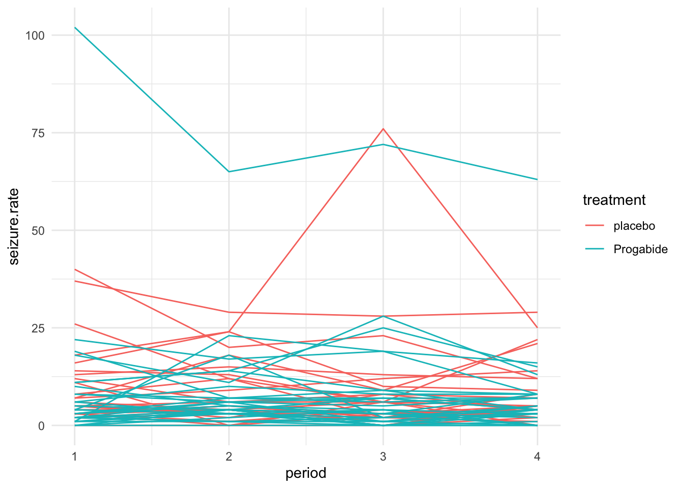
Figure 10.1: A spaghetti plot of the epilepsy data.
We can also plot the mean seizure rate at each time within each group as in Figure 10.2
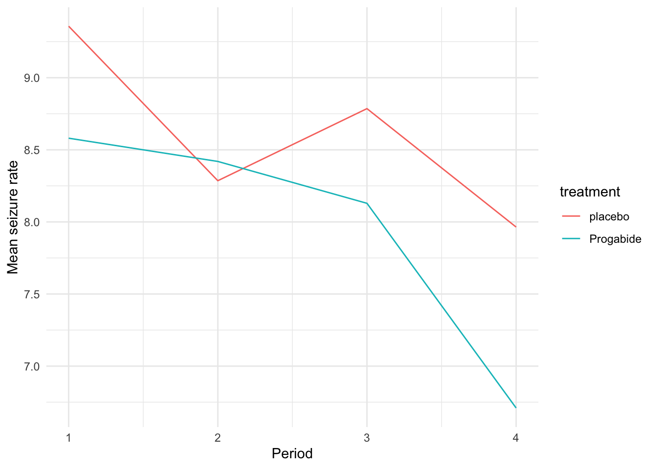
Figure 10.2: Mean seizure rate for each treatment group over time.
To make visualisation somewhat clearer, we can do a standardised spaghetti plot. In this plot, the observations are standardised within each time point. So, if \(x_{it}\) is the outcome for participant \(i\) and time \(t\), the standardised spaghetti plot would show
\[\frac{x_{it} - \bar{x}_t}{s_t} \]
where \(\bar{x}_t,\,s_t\) are the sample mean and SD at time \(t\). The standardised spaghetti plot for the epilepsy data is shown in Figure 10.3
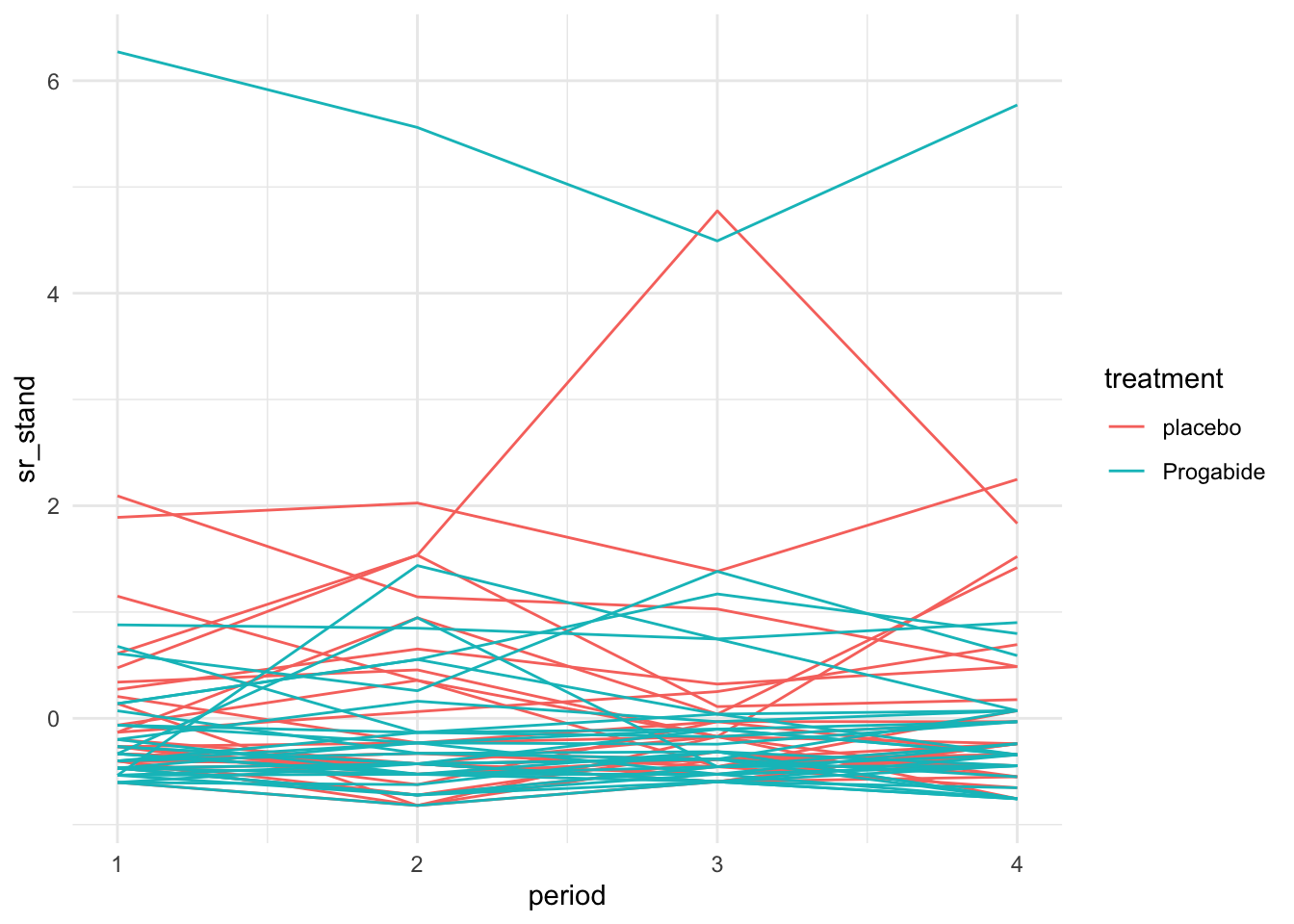
Figure 10.3: Standardised spaghetti plot for the epilepsy data.
10.2.1 Fitting a model
In longitudinal data the measurements are ‘clustered’ within each participant, in a semi-similar way to the participants being clustered within settings in Chapter 9. Each participant will have certain characteristics that don’t change through the duration of the trial, for example their age (at start), sex, disease history etc. Some of these characteristics we will record as part of the dataset, but this will not fully explain the correlation within measurements of the same participant.
We can also assume that, given the values of these covariates, the outcome of each participant has a slight (or mabye more than slight) propensity to be consistently either higher or lower than (or perhaps to be in line with) the mean. Therefore there will be a random effect associated with each participant. Because we are interested in how things evolve with time, we will also include time in the model.
The questions we want to answer are:
- What is the effect of the covariates (including treatment group) on the outcome?
- What is the effect of time on the outcome?
- Does the relationship between outcome and time vary for different groups of individuals?
10.2.2 The empty model
The very simplest mixed effects model we can fit is
\[\begin{equation} Y_{ij} = \beta_0 + u_{i} + \epsilon_{ij}. \tag{10.1} \end{equation}\]
In this model, \(Y_{ij}\) is the outcome for the \(i^{th}\) participant at time \(j\), \(\beta_0\) is a fixed effect representing the overall mean of the \(Y_{ij}\), \(u_i\) is the adjustment for the mean for participant \(i\) and \(\epsilon_{ij}\) is the residual. In this model we assume:
\[\begin{align*} u_{i} & \sim N\left(0,\,\sigma^2_{u}\right)\\ \epsilon_{ij}& \sim N\left(0,\,\sigma^2\right)\\ u_i&\perp \epsilon_{ij}. \end{align*}\]
This model is actually a one-way analysis of variance (ANOVA) model.
Example 10.3 We can fit the empty model for the epilepsy data via
## Linear mixed model fit by REML ['lmerMod']
## Formula: seizure.rate ~ 1 + (1 | subject)
##    Data: epilepsy
##
## REML criterion at convergence: 1651.1
##
## Scaled residuals:
##     Min      1Q  Median      3Q     Max
## -2.8126 -0.3264 -0.0797  0.1725  7.3634
##
## Random effects:
##  Groups   Name        Variance Std.Dev.
##  subject  (Intercept) 121.75   11.03
##  Residual              32.49    5.70
## Number of obs: 236, groups:  subject, 59
##
## Fixed effects:
##             Estimate Std. Error t value
## (Intercept)    8.263      1.484   5.569
The estimated average seizure.rate is shown in the Fixed effects section, and is 8.263. The estimated variance of the individual random effect term (\(u_i\) above) is 121.75, and the estimated residual variance is 32.49. These are both given in the Random effects section of the summary. We can use these values to estimate the ICC, which is now the correlation between repeated measures of the same individual:
\[\rho_{ICC} = \frac{s^2_B}{s^2_B + s^2_W} = \frac{121.75}{121.75+32.49} = 0.789.\]
This very high value of the ICC supports our choice of fitting a mixed effects model, rather than including only fixed effects.
Building up the model from this empty model basically involves including more fixed effects and random effects. Since we are concerned with longitudinal data, the obvious first thing to include is time. We can start by including a linear effect of time, so that the model in Equation (10.1) becomes
\[\begin{equation} Y_{ij} = \beta_0 + \gamma t_j + u_{i} + \epsilon_{ij}. \tag{10.2} \end{equation}\]
So that the coefficient \(\gamma\) describes the change in outcome with time.
We might go on to extend the model in Equation (10.2) by including some baseline covariates \(\mathbf{b}_{i}\) for participant \(i\) (these would be considered to be the same throughout the trial for participant \(i\)). Then our model becomes
\[\begin{equation} Y_{ij} = \beta_0 + \gamma t_j + \mathbf{b}_i^T\boldsymbol\beta + u_{i} + \epsilon_{ij}. \tag{10.3} \end{equation}\]
In Equation (10.3), the \(\mathbf{b}_i\) are being included as fixed effects, in much the same way we’re used to with linear models, and the corresponding vector of coefficients is \(\boldsymbol\beta\).
We will explore these models by fitting them to our epilepsy data.
## Including just time
epilepsy$period = as.numeric(epilepsy$period)
epi_1 = lmer(seizure.rate ~ period + (1|subject), data=epilepsy)

## Including more baseline covariates
epi_2 = lmer(seizure.rate ~ base + age + treatment + period + (1|subject), data=epilepsy)

pm1 = plot_model(epi_1)
pm2 = plot_model(epi_2)
grid.arrange(pm1, pm2, nrow=1)
Figure 10.4: Confidence intervals for fixed effects for the two fitted models.
In this example it appears that neither time nor the treatment have a significant effect on the seizure rate.
The final extension we’ll look at is if we think that different participants might change at different rates, all other things being equal. We can introduce a random effect \(\eta_i\) to allow the coefficient of time to vary between participants
\[\begin{equation} Y_{ij} = \beta_0 + \left(\gamma + \eta_i\right) t_j + \mathbf{b}_i^T\boldsymbol\beta + u_{i} + \epsilon_{ij}. \tag{10.4} \end{equation}\]
## Including just time
## Including more baseline covariates
epi_3 = lmer(seizure.rate ~ base + age + treatment + period + (period|subject), data=epilepsy)
summary(epi_3)
## Linear mixed model fit by REML ['lmerMod']
## Formula: seizure.rate ~ base + age + treatment + period + (period | subject)
## Data: epilepsy
##
## REML criterion at convergence: 1581.8
##
## Scaled residuals:
## Min 1Q Median 3Q Max
## -2.8224 -0.3265 -0.0224 0.2306 8.0745
##
## Random effects:
## Groups Name Variance Std.Dev. Corr
## subject (Intercept) 49.0650 7.0046
## period 0.2588 0.5088 -1.00
## Residual 31.8399 5.6427
## Number of obs: 236, groups: subject, 59
##
## Fixed effects:
## Estimate Std. Error t value
## (Intercept) -5.25307 4.45463 -1.179
## base 0.34338 0.03128 10.976
## age 0.15667 0.13409 1.168
## treatmentProgabide -0.82339 1.64777 -0.500
## period -0.48475 0.33514 -1.446
##
## Correlation of Fixed Effects:
## (Intr) base age trtmnP
## base -0.381
## age -0.914 0.188
## trtmntPrgbd -0.280 0.004 0.099
## period -0.221 0.000 0.000 0.000
## optimizer (nloptwrap) convergence code: 0 (OK)
## boundary (singular) fit: see help('isSingular')
Figure 10.5: Confidence intervals for model with same gradient for all participants (left) and for varying gradient (right).
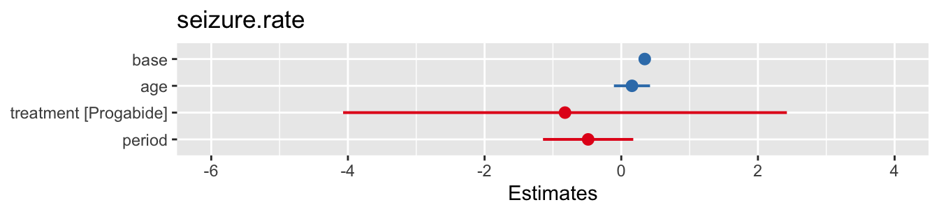
Figure 10.6: Confidence intervals for model with same gradient for all participants (left) and for varying gradient (right).
We see from the small variance for the random effect period that the gradients don’t vary very much at all, and indeed the coefficients of the fixed effects are very similar to those for a fixed gradient.
Summary
In these two lectures we’ve seen that random effects can be a useful way to take care of correlation between outputs for clusters of measurements.
This clustering can be because participants are from some natural group (eg. a school, a family, a hospital) or it can be because repeated measurements are taken of the same participant. In either case, we’d expect the measurements within one cluster to be more highly correlated than those from different clusters.