C Computer Practical 3 - Sample size by simulation
R practicalities - click here
There are many, many packages in R that implement methods for designing and analysing clinical trials (see a list at CRAN task view). We will look at some of these, and will also write our own code for some tasks. Remember that to install a package, you can do
If you have problems running R on your laptop, or on the university machines, the most foolproof way might be to use Github codespaces (thanks to Louis Aslett, who developed this). You may already be familiar with this from previous modules.
An advantage of this is that you can open the same codespace (the same instance of R) from any computer, so if you plan to work on things (for example your summative assignment, which will involve some R) from more than one computer, this might be ideal.
Here is a guide to getting set up.
A method for sample size calculation that has become increasingly popular in recent years is to use simulation. In simple terms, we write code that runs the trial many, many times in order to determine how many participants we need to achieve the power required. We can estimate the power by the proportion of simulated trials in which the null hypothesis was rejected.
Because the code necessarily works by fixing the number of participants and investigating the effect on the power of the trial, this is often referred to as power-calculation, but it is the same sample size issue, approached from a different angle. Arnold et al. (2011) gives a thorough, readable and interesting case study of the use of power simulation in a cluster randomised trial investigating different sanitation-related interventions in rural communities in Bangladesh.
The simulation approach has the following advantages over the formula-based methods presented in Sections 2 and 5:
- Transparency: If the data generating mechanism is made clear, then the assumptions behind the trial are also clear, and the simulation can be replicated by anyone. Reproducibility is a big issue in clinical trials.
- Flexibility: Whereas the methods in Sections 2 and 5 are limited to very specific circumstances, one can simulate arbitrarily complex or unusual trials. We can also explore the implications of the decisions we’ll have to make, such as how the allocation is made.
- Practice: This process requires us to perform our planned analysis at the planning stage (albeit likely in a simplified form), thus raising any potential issues early enough to adapt the statistical analysis plan.
Arguably the first and third advantages could also be true (though aren’t automatically) of a well-planned trial that used conventional sample size formulae, but the second is an advantage unique to simulation.
For most of this practical we will focus on continuous outcome variables, but the method can be applied to binary, survival or other kinds of data.
C.1 Power simulation for a t-test
Note: really we should be using more than 100 simulations, but so that the code runs in a sensible amount of time I’ve reduced the number. Feel free to increase it if you want to, but you’ll have to wait a little while for it to run.
We’ll start by taking a simulation approach to recreate the most ‘vanilla’ scenario, where we have a continuous outcome \(Y\) and wish to conduct a \(t\)-test on the outcome.
Recall that the sample size formula we found was Equation (2.4), shown again below:
\[N = \frac{2\sigma^2\left(z_\beta + z_{\frac{\alpha}{2}}\right)^2}{\tau_M^2},\] where \(N\) is the number of participants required in each trial arm, \(\sigma^2\) is the variance of the outcome \(Y\) in each group, and \(\tau_M\) is the minimum detectable effect size (or minimum clinically important difference), the smallest difference between \(\mu_C\) and \(\mu_T\) (the treatment arm means) that we want to be able to detect with significance level \(\alpha\) and power \(1-\beta\).
These variables give us all we need to simulate trial data. The model we will use here is
\[\begin{equation} Y_i= \sim \begin{cases} N\left(\mu,\;\sigma^2\right)&\;\text{ if participant }i\text{ is in group }C\\ N\left(\mu + \tau_M,\;\sigma^2\right)&\;\text{ if participant }i\text{ is in group }T. \end{cases} \tag{C.1} \end{equation}\]
Therefore, to simulate data from a trial like this, we need to specify values for \(\mu,\;\tau_M\) and \(\sigma^2\). We also need to specify the number of participants.
The steps for each simulation will be
- Simulate trial data using the distribution in Equation (C.1), for example using the function
rnorm - Conduct an un-paired, two-tailed \(t\)-test on the data
- Note whether \(H_0:\;\tau_M=0\) is rejected
Having done this for some number \(n_{sim}\) of simulations, we return the proportion of simulations in which \(H_0\) was rejected, and this is our power estimate.
If the power estimate is smaller than we would like, we increase the number of participants in our simulated trial data and try again. Conversely, we decrease the number of participants if the power estimate is larger than we need.
Exercise C.1 By generating data for group \(C\) and group \(T\) according to the distributions in Equation (C.1), conduct a power simulation for the trial scenario described in Example 2.1, with the aim of finding the number \(N\) of participants required in each arm for a power of 0.9 (\(\beta=0.1\)) and a confidence level of \(\alpha=0.05\). Recall that in that example we had minimum clinically important difference \(\tau_M = 3\) and pooled standard deviation estimate 8.
- How consistent are your results with the method we derived in Chapter 2?
- What issues does this raise around choosing a sample size?
If coding this up feels well outside your comfort zone, it’s fine to look at the solutions to see how I’ve done it - if it isn’t clear, please ask! Then you can try to adapt this approach in the future exercises
Click to reveal solution
Solution. The sensible first thing to do is to write a function that does this for general \(n_{sim},\,N,\,\mu,\,\sigma^2\) and \(\tau_M\). The very simplest way would be the following, where we generate \(N\) participants per arm, and their data.
ttest_sim = function(
    nsim,  # the number of simulations to use
    N,     # number of participants per trial arm
    mu,    # mean outcome (for group C / under H0)
    tm,    # minimum detectable effect size
    sd     # sd of outcome
){
  H0_reject_vec = rep(NA, nsim) # to store 1 if H0 rejected, 0 if fail to reject H0
  for (i in 1:nsim){
    # inside the loop we simulate a single trial with N in each group
    out_groupC = rnorm(N, mean=mu, sd=sd)
    out_groupT = rnorm(N, mean=mu + tm, sd=sd)
    ttest = t.test(
      out_groupC, out_groupT,
      alternative = "two.sided",
      var.equal = T, conf.level = 0.95)
    H0_reject_vec[i] = ifelse(ttest$p.value<0.05, 1, 0)
  }

  power.est = mean(H0_reject_vec)
  power.est
}
For a sanity check, we can put in the number we got from the equation in Section 2. To generate the data we need to specify a mean \(\mu\), but it doesn’t matter what it is (in this formulation at least!), so the number below is arbitrary.
## [1] 0.81and this is close to what we expect from the formula approach. To see how consistent this result is, we can see what happens over many sets of simulations
sim_vec1 = rep(NA, 100)
for (i in 1:100){
  sim_vec1[i] = ttest_sim(nsim=100, N=113, mu=5, tm=3, sd=8)
}
require(ggplot2)
ggplot(mapping = aes(sim_vec1)) + geom_histogram(bins=10)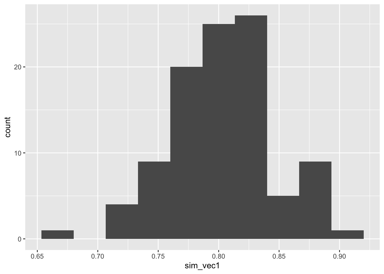
Figure C.1: Histogram of estimated powers from 100 lots of 100 simulations with N=113.
So although the mean power is around 0.8, as we expect, there is some variation.
To achieve \(1-\beta=0.9\) we need to increase \(N\). It turns out that around 155 participants in each arm gives a mean power of around 0.9.
sim_vec2 = rep(NA, 100)
for (i in 1:100){
  sim_vec2[i] = ttest_sim(nsim=100, N=155, mu=5, tm=3, sd=8)
}
ggplot(mapping = aes(sim_vec2)) + geom_histogram(bins=10)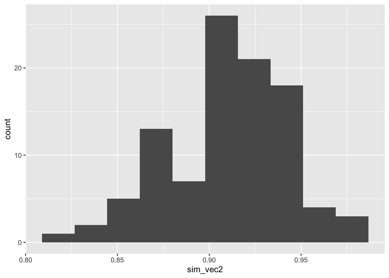
Figure C.2: Histogram of estimated powers from 100 lots of 100 simulations with N=155.
It is sensible to choose a number such that we are sufficiently confident of our study having the power we require. We may for example choose \(N\) so that the estimated power is at least 0.9 in some high proportion (say 90%) of the simulations.
A useful feature of the simulation approach is that it’s much easier to investigate what happens if the real data deviate in some way from the assumptions we’ve made.
Exercise C.2 Adapt your code (or my code) from Exercise C.1 to take into account the possibility of the outcome variance being different in the two groups. What is the effect on the estimated power if the outcome standard deviation in group \(T\) is 25% larger than the standard deviation in group \(C\)? What about if the outcome standard deviation is \(25\%\) smaller in group \(T\) than in group \(C\)?
Click to reveal solution
Solution. The change we need to make is to include a variance parameter for each group, rather than a common one. Note that we aren’t changing the t.test function to use unequal variances, as it is common practice to keep assuming equal variances, and actually these variances still aren’t that different.
ttest_sim2 = function(
    nsim,  # the number of simulations to use
    N,     # number of participants per trial arm
    mu,    # mean outcome (for group C / under H0)
    tm,    # minimum detectable effect size
    sdC,   # sd of outcome in group C
    sdT    # sd of outcome in group T
){
  H0_reject_vec = rep(NA, nsim) # to store 1 if H0 rejected, 0 if fail to reject H0
  for (i in 1:nsim){
    out_groupC = rnorm(N, mean=mu, sd=sdC)
    out_groupT = rnorm(N, mean=mu + tm, sd=sdT)
    ttest = t.test(
      out_groupC, out_groupT,
      alternative = "two.sided",
      var.equal = T, conf.level = 0.95)
    H0_reject_vec[i] = ifelse(ttest$p.value<0.05, 1, 0)
  }

  power.est = mean(H0_reject_vec)
  power.est
}
If the variances are equal, this gives the same as before (approximately)
## [1] 0.87However, if we increase the outcome variance in group \(T\) by 25%, things change:
## [1] 0.87sim_vec3 = rep(NA, 100)
for (i in 1:100){
sim_vec3[i] = ttest_sim2(nsim=100, N=155, mu=5, tm=3, sdC=8, sdT=10)
}
ggplot(mapping = aes(sim_vec3)) + geom_histogram(bins=10)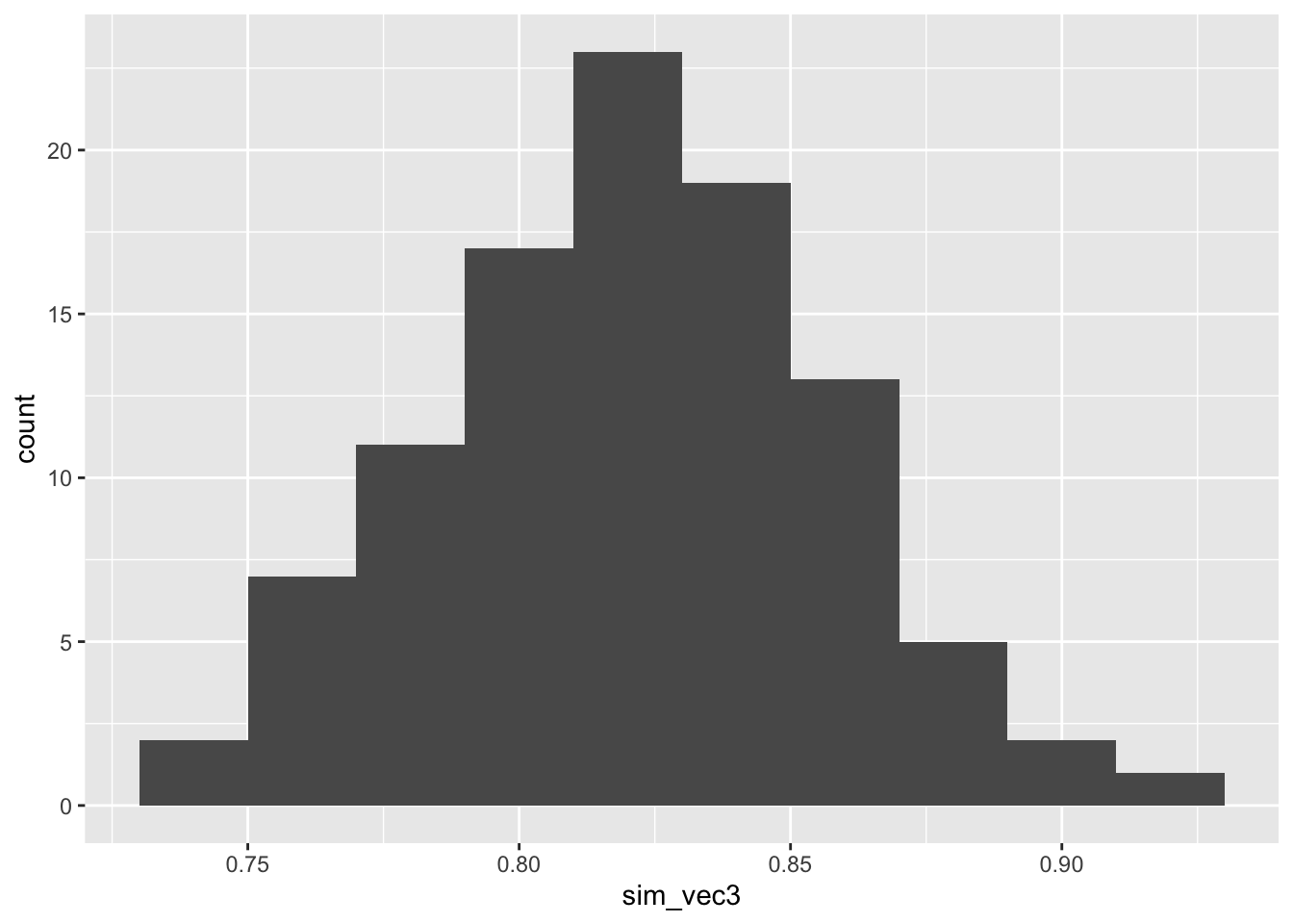
Figure C.3: Power estimates for 100 sets of 100 simulations with larger outcome SD in group T.
By contrast, if the outcome variance is lower (this is much less likely) then the power will be higher than calculated:
sim_vec4 = rep(NA, 100)
for (i in 1:100){
  sim_vec4[i] = ttest_sim2(nsim=100, N=155, mu=5, tm=3, sdC=8, sdT=6)
}
ggplot(mapping = aes(sim_vec4)) + geom_histogram(bins=10)
Figure C.4: Power estimates for 100 sets of 100 simulations with smaller outcome SD in group T
When using simulation in earnest, it is best to recreate as many features of the trial as we can, and this includes the allocation. If we were using a method that guaranteed [close to] exactly equal groups, then the above method is OK. However, this is not always the case. We will explore this in a fairly simple way.
Exercise C.3 Recreate the function from Exercise C.2, where the two groups have different variances. This time, simulate the data sequentially, using simple random sampling as the allocation method.
- What happens to the power distribution for the scenario we considered in that question?
- What happens for a much smaller \(N\), say \(N=25\)?
Click for solutions
Solution. For this method, we work through all \(2N\) participants sequentially, allocating them with equal probability to group \(C\) or \(T\). For readability, in these solutions the simulation of one trial is written as its own function, which is then implemented nsim times.
one_trial_srs = function(
    N,     # number of participants per trial arm
    mu,    # mean outcome (for group C / under H0)
    tm,    # minimum detectable effect size
    sdC,   # sd of outcome in group C
    sdT    # sd of outcome in group T
){
  ## Create empty vectors to contain output for groups C and T
  outC = integer()
  outT = integer()

  for (i in 1:(2*N)){
    # allocate using SRS
    arm = sample(c("C", "T"), size=1)
    # generate outcome according to groups' distributions
    if (arm == "C"){
      outi = rnorm(1, mean=mu, sd=sdC)
      outC = c(outC, outi)
    } else if (arm == "T"){
      outi = rnorm(1, mean=mu+tm, sd=sdT)
      outT = c(outT, outi)
    }
  }
  # conduct t-test for this trial
  t.test(x=outC, y=outT,
         alternative = "two.sided", paired=F,
         var.equal=T, conf.level=0.95)
}

ttest_sim_srs = function(
    nsim,  # the number of simulations to use
    N,     # number of participants per trial arm
    mu,    # mean outcome (for group C / under H0)
    tm,    # minimum detectable effect size
    sdC,   # sd of outcome in group C
    sdT    # sd of outcome in group T
){
  H0_reject_vec = rep(NA, nsim) # to store 1 if H0 rejected, 0 if fail to reject H0

  for (i in 1:nsim){
    trial_i = one_trial_srs(N, mu, tm, sdC, sdT)
    H0_reject_vec[i] = ifelse(trial_i$p.value<0.05, 1, 0)
  }

  power.est = mean(H0_reject_vec)
  power.est
}

ttest_sim_srs(nsim=100, N=155, mu=5, tm=3, sdC=8, sdT=10)
## [1] 0.89To see the distribution for many simulations, we can do
sim_vec5 = rep(NA, 100)
for (i in 1:100){
  sim_vec5[i] = ttest_sim_srs(nsim=100, N=155, mu=5, tm=3, sdC=8, sdT=10)
}
ggplot(mapping = aes(sim_vec5)) + geom_histogram(bins=10)
Figure C.5: Power estimates for 100 sets of 100 simulations with N=155 with larger outcome SD in group T, with SRS allocation.
and we see that the spread is much higher than when we had two exactly equal groups, as in Figure C.3.
If \(N\) is smaller, the variance in the power estimates will be higher, because the potential for imbalance will be greater.
C.2 Power simulation for ANCOVA
In our analysis section we learned that the ANCOVA model is much more efficient and flexible than a t-test, so now we’ll simulate our data with that analysis method in mind.
We’ll write our data-generating model for the outcome \(X_i\) as
\[ \begin{aligned} x_i & = \mu + \rho \left(b_i - \mu_B\right) + \epsilon_i & \text{ in group C}\\ x_i & = \mu + \tau + \rho \left(b_i - \mu_B\right) + \epsilon_i & \text{ in group T}&. \end{aligned} \] where \(\epsilon_i\sim N\left(0,\,\sigma^2_{\epsilon}\right)\). Now, we need to generate a value of the baseline measurement \(b_i\) for each patient, and specify values for \(\mu\) (the mean outcome in group C / under \(H_0\)), \(\mu_B\) (the mean baseline measurement), \(\tau_M\) (the minimum detectable effect size, taking the place of \(\tau\) in the above equation), \(\rho\) (the correlation between baseline and outcome measurement) and \(\sigma^2_{\epsilon}\). Some of these are quantities that might be well-understood from the literature, but others are more speculative.
Exercise C.4 Conduct a power simulation by simulating 100 participants in each group with the distributions above, where
- \(b_i\sim N\left(\mu_B,\,8^2\right)\) for all \(i\)
- \(\epsilon_i\sim N\left(0,\,6^2\right)\) for all \(i\)
- \(\mu = 60\)
- \(\rho = 0.65\)
- \(\mu_B = 50\)
- \(\tau_M = 3\)
For now, assume that the participants are allocated by simple random sampling. How do your results compare with the results from Exercise C.3, and why?
Click for solutions
Solution. Now that we have a baseline variable to keep track of, we should create a data frame of participants as we generate them.
## Function to simulate one trial (with ANCOVA analysis)
ancova_trial_srs = function(
    N,       # Number of participants per group
    mu_B,    # baseline mean
    mu,      # outcome mean (control group / H_0)
    rho,     # correlation between baseline and outcome
    tm,      # minimum detectable effect size
    sd_eps,  # SD of error
    sd_B     # SD of baseline measurement
){
  ## Empty data frame for trial data
  trial_mat = matrix(NA, ncol=3, nrow=2*N)
  trial_df = data.frame(trial_mat)
  names(trial_df) = c("baseline", "arm", "outcome")

  for (i in 1:(2*N)){
    bas_i = rnorm(1, mean=mu_B, sd=sd_B)
    trial_df$baseline[i] = bas_i
    alloc_i = sample(c("C", "T"), 1) # Using SRS in this function
    trial_df$arm[i] = alloc_i
    eps_i = rnorm(1, mean=0, sd=sd_eps)
    if(alloc_i == "C"){
      out_i = mu + rho*(bas_i - mu_B) + eps_i
    } else if (alloc_i == "T"){
      out_i = mu + tm + rho*(bas_i - mu_B) + eps_i
    }
    trial_df$outcome[i] = out_i
  }
  model.fit = lm(outcome ~ baseline + arm, data=trial_df)
  summary(model.fit)
}

## Function to simulate many trials (with ANCOVA analysis)

ancova_sim_srs = function(
    nsim,  # the number of simulations to use
    N,       # Number of participants per group
    mu_B,    # baseline mean
    mu,      # outcome mean (control group / H_0)
    rho,     # correlation between baseline and outcome
    tm,      # minimum detectable effect size
    sd_eps,  # SD of error
    sd_B     # SD of baseline measurement
){
  H0_reject_vec = rep(NA, nsim) # to store 1 if H0 rejected, 0 if fail to reject H0

  for (i in 1:nsim){
    trial_i = ancova_trial_srs(N, mu_B, mu, rho, tm, sd_eps, sd_B)
    H0_reject_vec[i] = ifelse(trial_i$coefficients[3,4]<0.05, 1, 0)
  }

  power.est = mean(H0_reject_vec)
  power.est
}
sim_vec6 = rep(NA, 100)
for (i in 1:100){
sim_vec6[i] = ancova_sim_srs(nsim=100, N=90, mu_B=50, mu=60,
rho=0.65, tm=3, sd_eps=6, sd_B = 8)
}
ggplot(mapping = aes(sim_vec6)) + geom_histogram(bins=10)
Figure C.6: Power estimates for 100 sets of 100 simulations with larger outcome SD, with SRS allocation, with \(N=75\), assuming an ANCOVA analysis.
The power is much higher than for our t-test simulation with \(N=100\). This is because the variance of the treatment effect estimate is lower for ANCOVA for the t-test (by a factor of \(1-\rho^2\)), as we saw in Section 4.3.1.2.
C.3 Conclusion
We could extend this in many ways to better understand the uncertainty around the power for a given sample size. For example:
- Trying different allocation methods
- Incorporating uncertainty around quantities like \(\mu,\,\mu_B,\,\rho\) etc.
If you still have time you might like to explore one of these ideas, or make a start on Practical 4, as there’s a lot to cover!