2 Sample size for a normally distributed primary outcome variable
For most of this module, we’ll focus on randomised controlled trials (RCTs). These have mainly been used for clinical applications (for example, to test a particular drug), but have also recently become popular ways to test interventions in areas such as education and policing.
Having laid the groundwork in Chapter 1, we now go on to some more technical details. In this Chapter, we focus on the ‘vanilla’ scenario, where we have a trial with two arms, and our unit of randomization is individuals. At first we will focus only on continuous outcomes, but in later weeks we will go on to think about binary and time-to-event data.
The topics we cover fall into the categories of ‘before the trial’ (design and planning) or ‘after the trial’ (analysis), although as we’ll see there is some interaction between these stages.
The first big question asked of a trial statistician is usually how many participants does the trial need in order to be viable: the sample size. We will clarify what is meant by ‘viable’ later in this section.
Broadly speaking, there are two (opposing) ethical issues around sample size:
- If we don’t recruit enough patients, then we may not gather enough evidence to draw any conclusion about the research question (ie. whether there is a treatment effect). As well as being scientifically disappointing, this is unethical. To conduct the trial, some of the patients will have been subject to an inferior treatment (assuming one treatment was actually better), and if there is no conclusion then this was effectively for no purpose.
- If we recruit too many patients (ie. we would be sufficiently likely to reach a conclusion with fewer) then we have subjected more patients than necessary to an inferior treatment (assuming one treatment was better), and have probably taken up more time and resources than was necessary.
It is therefore important to think about this issue carefully. We’ve framed the question in quite a woolly way so far, but now we’ll start to think more carefully.
2.1 The treatment effect
In Section 1.2 we discussed the need to settle on a primary outcome variable. One reason this is important is that we base our sample size calculations on the primary outcome variable.
Definition 2.1 Suppose our primary outcome variable is \(X\), which has mean \(\mu\) for the control group and mean \(\mu + \tau\) for the treatment group. The variable \(\tau\) is the treatment effect. The goal of our RCT is to learn about \(\tau\). The larger \(\tau\) is (in magnitude), the more pronounced the effect of the intervention.
This problem is usually framed as a hypothesis test, where the null hypothesis is that \(\tau=0\).
2.2 Reminder: hypothesis tests (with a focus on RCTs)
When performing a hypothesis test, what we are aiming to find is the P-value.
Definition 2.2 The P-value is the probability of obtaining a result as extreme as or more extreme (ie. further away from the null hypothesis value) than the one obtained given that the null hypothesis is true.
Put simply, the P-value is a measure of the probability of obtaining whatever result (eg. treatment effect) we have have found simply by random chance, when in fact there is no treatment effect (ie. \(\tau=0\)). We use the data to calculate a test statistic, whose distribution under the null hypothesis we understand (given some assumptions), and this allows us to find the P-value.
Generally, a P-value below \(\alpha = 0.05\) is accepted as sufficient evidence to reject the null hypothesis, although in clinical settings the threshold can often be smaller (eg. \(\alpha = 0.01\)). It is conventional to present the P-value by simply saying whether it is smaller than some threshold (often 0.05), rather than giving the exact value.
Definition 2.3 The threshold for the P-value below which the results are considered ‘significant’ is known as the significance level of the test, and is generally written \(\alpha\) (as above).
This use of a significance level is (in part) a legacy from early days when computers were rare and values were looked up in \(t\)-tables (or similar). Now that it is very simple to find the exact P-value, it is becoming more and more common to report the actual number. Indeed, there is a big difference between \(p=0.049\) and \(p=0.000049\).
2.2.1 One-tailed or two-tailed?
It is highly likely that the scientists running the trial will have a strong idea of the likely ‘direction’ of the treatment effect. Assuming that a larger value of the primary outcome variable \(X\) is good, they will expect / hope for a positive value of the treatment effect \(\tau\) (or be prepared to accept that the effect might be minimal).
It would therefore be tempting to perform a one-sided test, with
\[\begin{align*} H_0\,&:\, \tau=0\\ H_1\,&:\, \tau>0. \end{align*}\]
For example, suppose our test statistic \(t\) has a \(t\) distribution with 31 degrees of freedom and we obtain a value of 2, as shown in Figure 2.1. In this case our P-value is \(1 - F_t\left(2, df=31\right)= 0.0272\) (where \(F_t\left(\cdot\right)\) is the cumulative distribution function of the \(t\) distribution) , and the result would be considered significant at the 0.05 level.
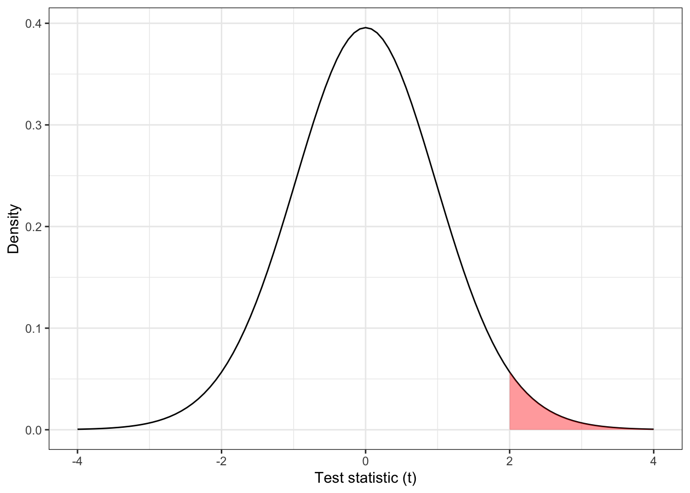
Figure 2.1: The distribution \(t_{31}\), with the area corresponding to \(t > 2\) shaded.
For a large positive value of \(t\), we obtain a small P-value, and reject \(H_0\), concluding that the intervention is effective (in a good way). However, what if we obtain a large negative value of \(t\)? In this one-sided set-up, there is no value of \(t<0\) that would give a significant result; negative values of \(t\) are simply considered consistent with \(H_0\), and there is no mechanism to conclude that an intervention has a significantly negative effect.
For this reason, we always conduct two sided hypothesis tests, with
\[\begin{align*} H_0\,&:\, \tau=0\\ H_1\,&:\, \tau\neq 0. \end{align*}\]
In this scenario, Figure 2.1 is replaced by the plot shown in Figure 2.2, where values of \(t\) with \(t<-2\) are considered ‘equivalent’ to those with \(t>2\), in the sense of how unlikely they are under \(H_0\).
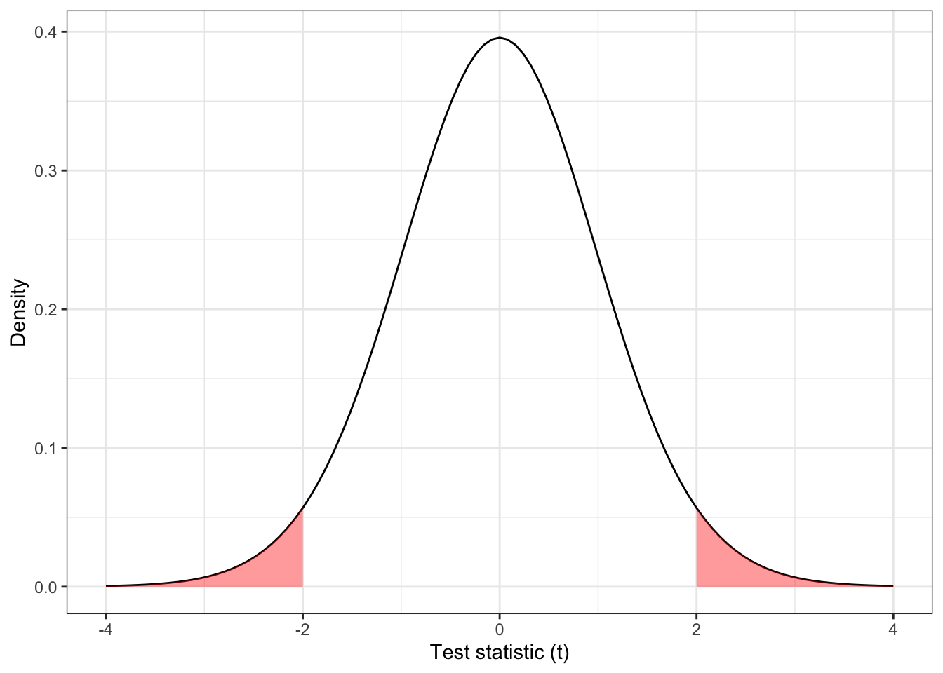
Figure 2.2: The distribution \(t_{31}\), with the area corresponding to \(|t| > 2\) shaded.
The P-value for the two-sided test as shown in Figure 2.2 is
\[ F\left(-2, df=31\right) + \left[1 - F\left(2, df=31\right)\right] = 2\times{0.0272} = 0.0543\] and the result is no longer significant at the 0.05 level. Throughout this course, we will always assume two-tailed tests.
2.2.2 Insignificant results
If our P-value is relatively large, say 0.3 or 0.5 (or really, greater than \(\alpha\)), then our result is not at all unlikely (or sufficiently unlikely) under the null hypothesis, and provides insufficient evidence to reject \(H_0.\) However, it is not inconsistent with the existence of a treatment effect, so we don’t say there is evidence to accept \(H_0\). One can imagine that if the true treatment effect \(\tau\) were tiny, many trials would fail to find evidence to reject \(H_0\). However, if our sample size were sufficiently large, we should be able to detect it. Conversely, if \(\tau\) is very large, even a relatively small sample size is likely to provide enough evidence to reject \(H_0\).
A non-significant P-value means that our results are consistent with the null hypothesis \(\tau=0\), but they are also consistent with some small treatment effect, and therefore we can’t conclude very much. The key issue is, what size of treatment effect do we care about? We must ensure that our sample size is large enough to be sufficiently likely to detect a clinically meaningful treatment effect.
We are being vague for now, but this is a key issue in determining an appropriate sample size.
2.3 Constructing a measure of effect size
Let’s say we are recruiting participants into two groups: group \(T\) will be given the new treatment (they will sometimes be referred to as the treatment group or treatment arm, or alternatively the intervention group) and group \(C\) will be given the control (they are the control group or control arm).
Suppose that we have \(n\) patients in group \(C\), and \(m\) in group \(T\). The primary outcome variable \(X\) is normally distributed with mean \(\mu\) in group C (the control group) and mean \(\mu+\tau\) in group T (the intervention group), and common standard deviation \(\sigma\). So
\[\begin{align*} X & \sim N\left(\mu, \sigma^2\right) \text{ in group }C\\ X & \sim N\left(\mu + \tau, \sigma^2\right) \text{ in group }T. \end{align*}\]
We are testing the null hypothesis \(H_0: \tau=0\) against the alternative hypothesis \(H_1: \tau\neq{0}\).
Using the data obtained in the trial, we will be able to obtain sample means \(\bar{x}_C\) and \(\bar{x}_T\) from each group, and a pooled estimate of the standard deviation
\[ s = \sqrt{\frac{\left(n-1\right)s_C^2 + (m-1)s_T^2}{n+m - 2}}, \] where \(s_C\) and \(s_T\) are the sample standard deviations for groups \(C\) and \(T\) respectively, for example
\[ s_C = \sqrt{\frac{\sum\limits_{i=1}^n{\left(x_i - \bar{x}_C\right)^2}}{n-1}}. \]
Using these values we can compute
\[D = \frac{\bar{x}_T - \bar{x}_C}{s\sqrt{\frac{1}{n} + \frac{1}{m}}}\] as a standardised measure of the effect \(\tau\).
Theorem 2.1 Under \(H_0\), and the model we’ve specified, \(D\) has a \(t\)-distribution with \(n+m-2\) degrees of freedom.
Proof. Under \(H_0\) the \(x_i\) are iid \(N\left(\mu,\;\sigma^2\right)\), and so
\[\begin{align*} \bar{x}_C & \sim{N\left(\mu, \frac{\sigma^2}{n}\right)}\\ \bar{x}_T & \sim{N\left(\mu, \frac{\sigma^2}{m}\right)} \end{align*}\]
and therefore
\[ \bar{x}_T - \bar{x}_C \sim{N \left(0, \sigma^2\left[\frac{1}{n} + \frac{1}{m}\right] \right)}\]
and \[ \frac{\bar{x}_T - \bar{x}_C}{\sigma \sqrt{\frac{1}{n}+\frac{1}{m}}} \sim{N\left(0,1\right)}.\]
We know that for \(x_1,\ldots,x_n,\sim N\left(\mu,\sigma^2\right)\) for some arbitrary \(\mu\) and \(\sigma^2\),
\[\frac{1}{\sigma^2}\sum\limits_{i=1}^n\left(x_i - \bar{x}\right)^2 \sim{\chi^2_{n-1}},\] and so we have
\[\begin{align*} \frac{n-1}{\sigma^2}s_C^2 & \sim \chi^2_{n-1}\\ \frac{m-1}{\sigma^2}s_T^2 & \sim \chi^2_{m-1}\\ \text{and} &\\ \frac{1}{\sigma^2}\left[\left(n-1\right)s_C^2 + \left(m-1\right)s_T^2\right] & = \frac{n+m-2}{\sigma^2}s^2\\ &\sim \chi^2_{n+m-2}. \end{align*}\]
The definition of a \(t\)-distribution is that if \(Z\sim N\left(0,1\right)\) and \(Y \sim{\chi^2_n}\) then
\[X = \frac{Z} {\sqrt{\frac{Y}{n}}} \sim{t_n},\] that is \(X\) has a \(t\) distribution with \(n\) degrees of freedom.
Plugging in our \(N\left(0,1\right)\) variable for \(Z\) and our \(\chi^2_{n+m-2}\) variable for \(Y\), we have
\[\begin{align*} \frac{\frac{\bar{x}_T - \bar{x}_C}{\sigma\sqrt{\frac{1}{n} + \frac{1}{m}}}}{\sqrt{\left(\frac{n+m-2}{\sigma^2}s^2\right) \bigg/ \left(n+m-2\right)}} & = \frac{\bar{x}_T - \bar{x}_C}{\sigma\sqrt{\frac{1}{n} + \frac{1}{m}}} \bigg/ \frac{s}{\sigma} \\ & = \frac{\bar{x}_T - \bar{x}_C}{s\sqrt{\frac{1}{n} + \frac{1}{m}}} \\ & = D \end{align*}\]
and therefore \(D\) has a \(t\) distribution with \(n+m-2\) degrees of freedom.
We can therefore use \(D\) as our test statistic; if \(D\) is such that
\[ |D| > t_{n+m-2}\left(\alpha/2\right)\] where \(t_{n+m-2}\left(\cdot\right)\) is the function such that \(P\left(T>t_{df}\left(\xi\right)\right) = \xi\) when \(T \sim{t_{df}}\) then we can reject \(H_0\).
In practical terms, for more than around 40 degrees of freedom, the \(t\) distribution is indistinguishable from the normal distribution, and since it is rare to have fewer than 40 participants in an RCT, we use a normal approximation in what follows, and a difference is significant at the \(100\left(1-\alpha\right) \%\) level if \(|D| > z_{\alpha/2}\), where \(z\) are standard normal quantile values. For example, for \(\alpha=0.05\) we have \(z_{\alpha/2} = 1.960\), since the probability of a standard normal variable exceeding this value is 0.025.
So, if we have run a trial, and have obtained \(n\) values of \(X\) from group \(C\) and \(m\) values of \(X\) from group \(T\), we can compute \(D\). If \(D\) lies outside the interval \(\left[-z_{\alpha/2}, z_{\alpha/2}\right]\) then we reject \(H_0\).
This is equivalent to \(\bar{x}_T - \bar{x}_C\) falling outside the interval
\[\left[-z_{\alpha/2}s\sqrt{\frac{1}{n} + \frac{1}{m}},\; z_{\alpha/2}s\sqrt{\frac{1}{n} + \frac{1}{m}} \right]. \]
Brief aside on notation
We’ll see a lot of the notation \(z_{\alpha/2}\) and similar, so to clarify:
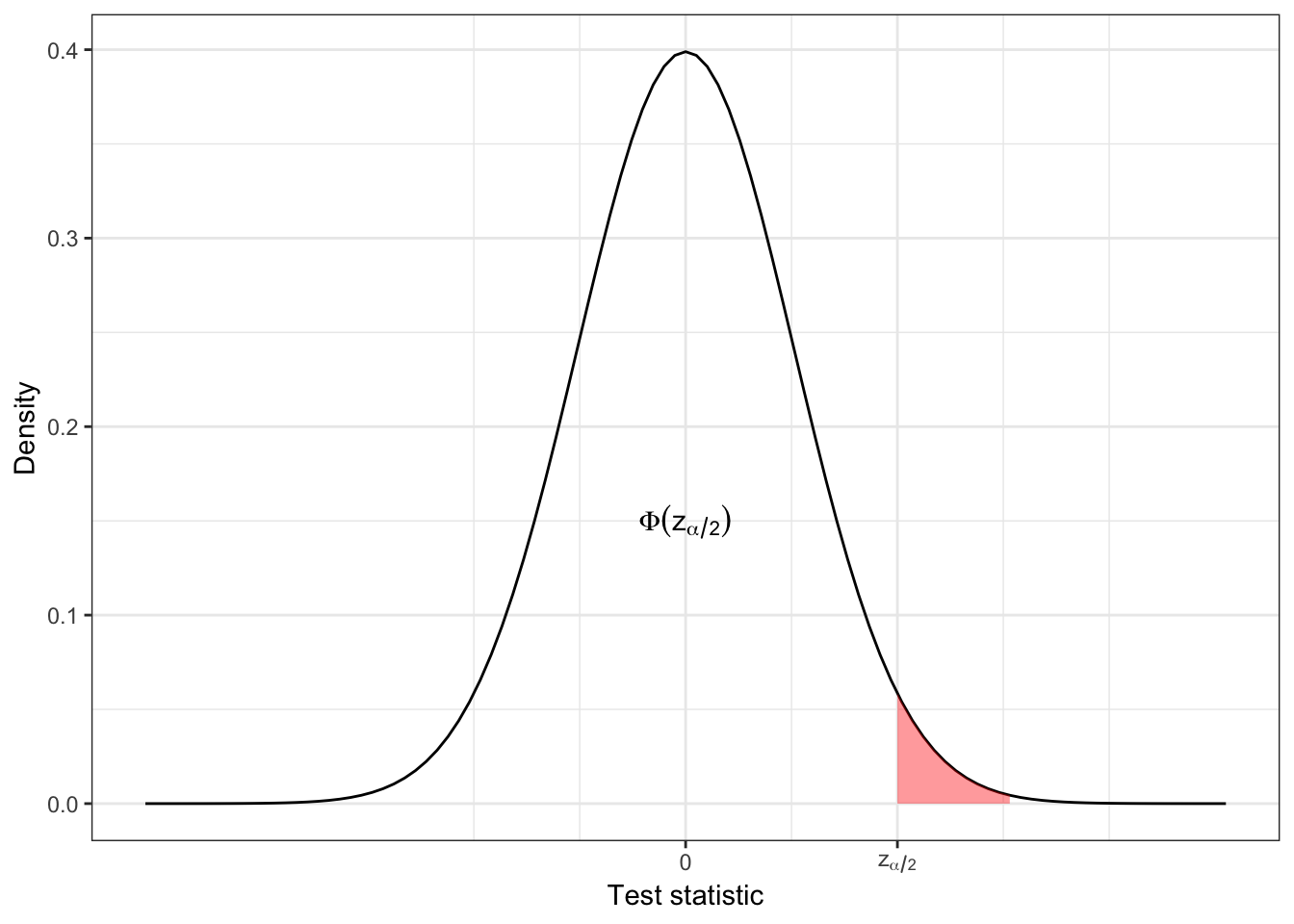
In R, we have \(\Phi\left(z_{\alpha/2}\right) = \texttt{pnorm}\left(z_{\alpha/2}\right)\) and \(z_{\alpha/2} = \texttt{qnorm}\left(\Phi\left(z_{\alpha/2}\right)\right)\). qnorm is the quantile and pnorm is the cumulative distribution function. So,
\[\frac{\alpha}{2} = 1 - \Phi\left(z_{\alpha/2}\right).\]
We have constructed our whole argument under the assumption that \(H_0\) is true, and that the probability of such a value is therefore \(\alpha\). We want this probability to be small, since it constitutes an error; \(H_0\) is true, but our value of \(D\) (or the difference in means) leads us to reject \(H_0\). This is sometimes called the ‘type I’ error rate. But what if \(H_0\) is false?
2.4 Power: If \(H_0\) is false
We have constructed things so that if \(H_0\) is true, we have a small probability of rejecting \(H_0\). But if \(H_0\) is false, and \(\tau\neq{0}\), we want our test to have a high probability of rejecting \(H_0\).
Definition 2.4 The power of a test is the probability that we reject \(H_0\), given that \(H_0\) is false. The power function depends on the value of \(\tau\) and is
\[\Psi\left(\tau\right) = \Pr\left(\text{Reject } H_0\mid{\tau\neq{0}}\right) = 1 - \beta.\] We therefore also have
\[\beta = \Pr\left(\text{Fail to reject } H_0\mid{\tau\neq{0}}\right). \]
We call \(\beta\) the type II error rate.
If you find the notation confusing (as I do!) then it might be helpful to remember that both \(\alpha\) and \(\beta\) are error rates - probabilities of coming to the wrong conclusion. It is common to talk in terms of \(\alpha\), the significance level, (which will be a low number, often 0.05) and of \(1-\beta\), the power (which will be a high number, often 0.8). I’ve found though that it is not uncommon to find people refer to \(\beta\) (rather than \(1-\beta\)) as the power. If in doubt, keep in mind that we require \(\alpha,\;\beta \ll 0.5\). It is also common to use percentages: a significance level of \(\alpha=0.05\) can also be referred to as “the 95% level”, and \(\beta=0.2\) is the same as a “power of 80%”. When using percentages, we talk in terms of the amount of time we expect the test to come to the correct conclusion.
If you notice any mistakes in these notes along these (or other!) lines, please point them out.
Under \(H_1\), we have
\[D = \frac{\bar{x}_T - \bar{x}_C}{s\sqrt{\frac{1}{n} + \frac{1}{m}}},\]
and therefore (approximately)
\[D \sim{N\left(\frac{\tau}{\sigma\lambda\left(n,m\right)}, 1\right)},\] where \(\lambda\left(n,m\right) = \sqrt{\frac{1}{n}+\frac{1}{m}}\).
Figure 2.3 shows the distribution of \(D\) under \(H_0\) and \(H_1\) for some arbitrary (non-zero) effect size \(\tau\). The turquoise bar shows the ‘acceptance region’ of \(D\), ie. the range of observed values of \(D\) for which we will fail to reject \(H_0\). We see that this contains 95% of the area of the \(H_0\) distribution (we have set \(\alpha = 0.05\) here), so under \(H_0\), we have a 0.95 probability of observing a value of \(D\) that is consistent with \(H_0\). This could easily generalise to another value of \(\alpha\).
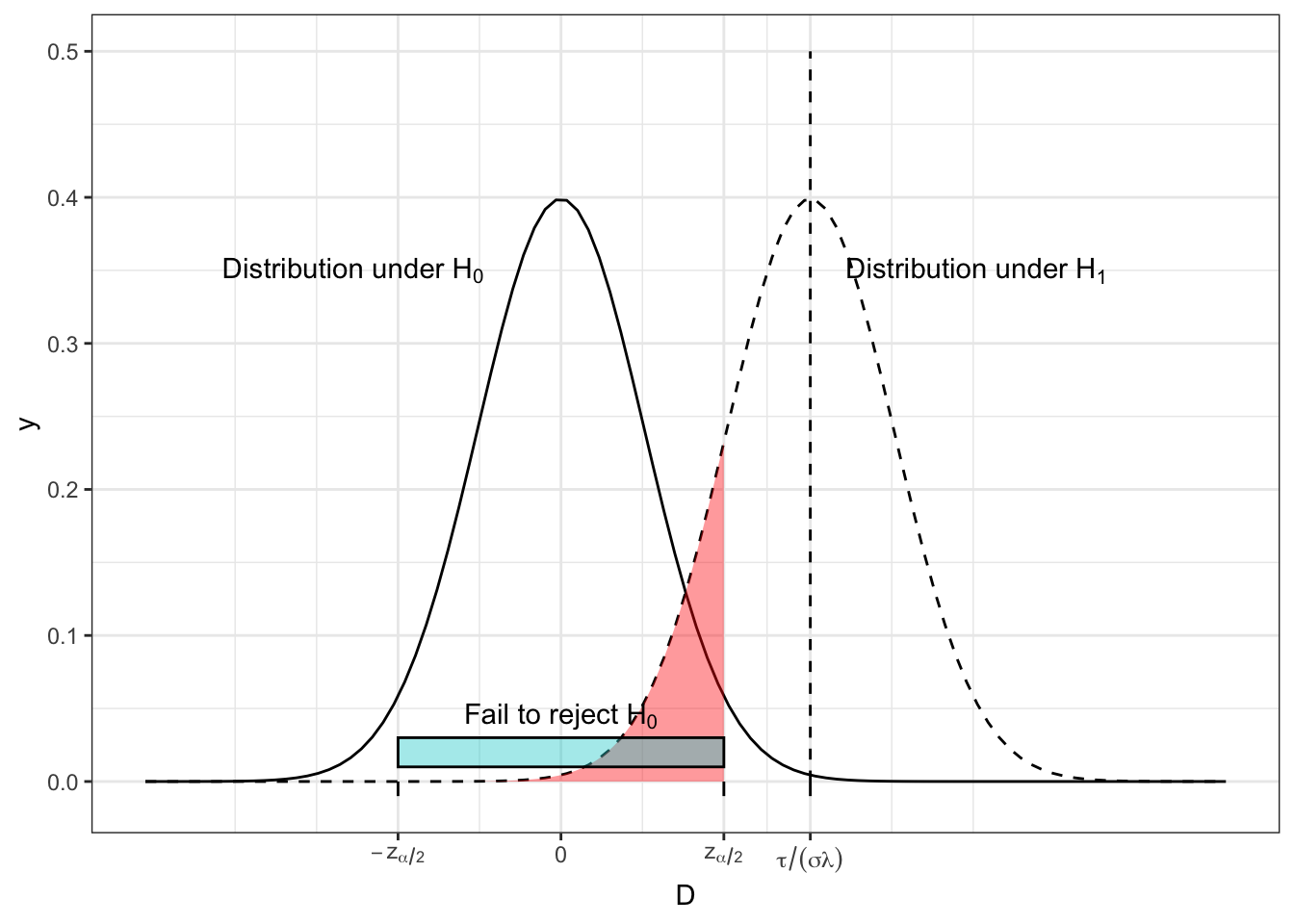
Figure 2.3: The distribution of \(D\) under both \(H_0\) and \(H_1\) for some arbitrary values of effect size, population variance, \(n\) and \(m\), with the region in which we fail to reject \(H_0\) shown by the turquoise bar and the red shading.
However, if \(H_1\) is true, and \(\tau\neq{0}\), there is a non-zero probability of observing a value of \(D\) that would lead us to fail to reject \(H_0\). This is shown by the area shaded in red, and it has area \(\beta\). One minus this area (ie. the area under \(H_1\) that leads us to reject \(H_0\)) is the power, \(1-\beta\).
We can see that if the distributions have better separation, as in Figure 2.4, the power becomes greater. This can be as a result of a larger \(\tau\), a smaller \(\sigma\) or a smaller \(\lambda\) (therefore larger \(m\) and/or \(n\)).
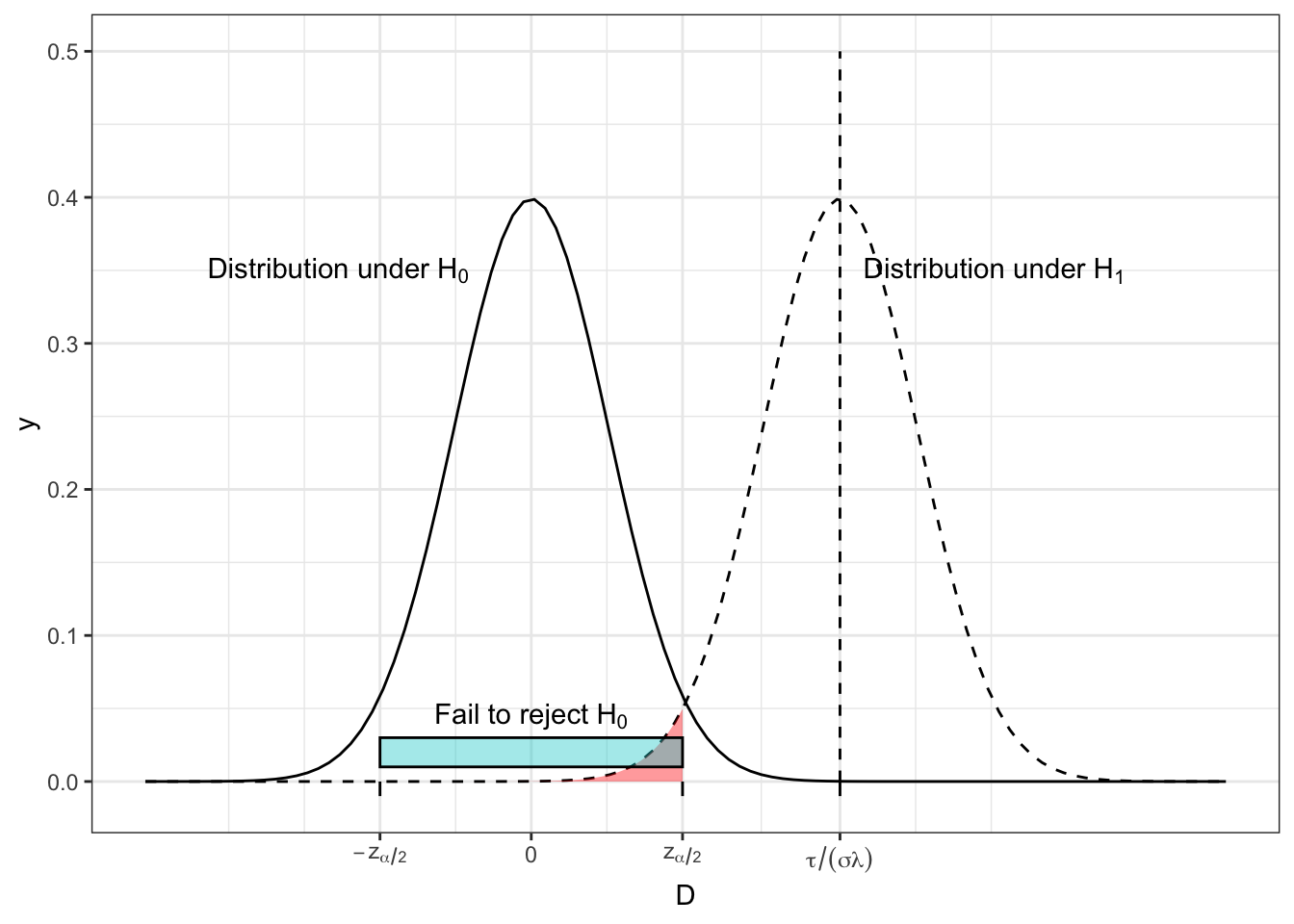
Figure 2.4: The distribution of D under both \(H_0\) and \(H_1\) for some arbitrary values of effect size, population variance, \(n\) and \(m\), with the region in which we fail to reject \(H_0\) shown by the turquoise bar and the red shading.
For given values of \(\alpha\), \(\sigma\) and \(\lambda\left(n,m\right)\), we can calculate the power as a function of \(\tau\) by finding the area of the distribution of \(D\) under \(H_1\) for which we accept \(H_1\).
\[\begin{equation} \Psi\left(\tau\right) = 1-\beta = \left[1 - \operatorname{\Phi}\left(z_{\frac{\alpha}{2}} - \frac{\tau}{\sigma\lambda}\right)\right] + \operatorname{\Phi}\left(-z_{\frac{\alpha}{2}} - \frac{\tau}{\sigma\lambda}\right) \tag{2.1} \end{equation}\]
The first term in Equation (2.1) is the area in the direction of \(\tau\). In Figures 2.3 and 2.4 this is the region to the right of the interval for which we fail to reject \(H_0\), ie. where \[D > z_{\frac{\alpha}{2}}.\]
The second term in Equation (2.1) represents the area away from the direction of \(\tau\), ie. a value of \(D\) such that
\[ D < - z_{\frac{\alpha}{2}},\] assuming without loss of generality that \(\tau>0\).
Figure 2.5 shows the power function \(\Psi\left(\tau\right)\) for \(\tau\) in units of \(\sigma\) (or you could think of this as for \(\sigma=1\)), for three different pairs of values of \(n\) and \(m\) (remember that these enter the power function via \(\lambda\)) with \(\alpha=0.05\). We see that in general the power is higher for larger sample sizes, and that of the two designs where \(n+m=200\), the balanced one with \(n=m=100\) achieves the greatest power.
In general, the probability of rejecting \(H_0\) increases as \(\tau\) moves away from zero.
Notice also that all the curves pass through the point \(\tau=0,\,\beta=0.05\). Since \(\tau=0\) corresponds to \(H_0\) being true, it makes sense that the probability of rejecting the \(H_0\) is the significance level \(\alpha\).
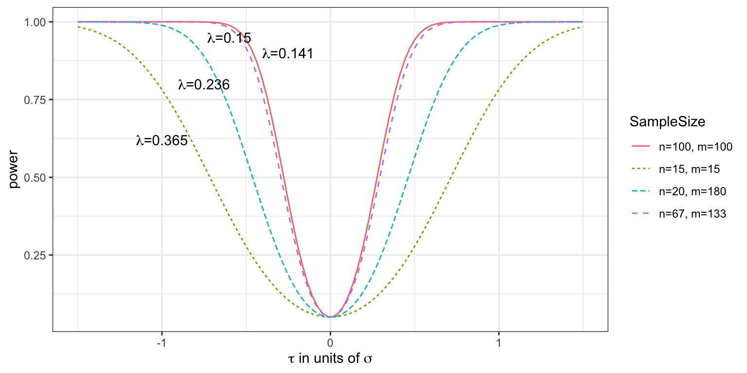
Figure 2.5: Power curves for various values of \(n\) and \(m\), with effect size in units of standard deviation, given a type I error rate of 0.05.
It is common to think of the effect size in units of \(\sigma\), as we have done here. This makes results more intuitive, since we don’t need to have a good knowledge of the actual outcome variable to know what is a small or large effect size. It is also helpful in situations where the population standard deviation is not well understood, since the trial can be planned with this sort of effect size in mind. To denote the effect size in units of \(\sigma\), we will write \(\tau_\sigma\), although in practice it is more usual to give both the same notation. In a medical setting we will often have an estimate for \(\sigma\) (for example from previous studies).
2.5 A sample size formula
Equation (2.1) allows us to find any one of \(\tau_\sigma,\,\alpha,\,\beta\) and \(\lambda\left(n,m\right)\) given values for the others.
Values for \(\alpha\) and \(\beta\) are often specified by those planning the trial as around \(\alpha \in \left[0.01,0.05\right],\,1-\beta\in\left[0.8,0.9\right]\). The remaining two values, \(\tau_\sigma\) and \(\lambda\left(n,m\right)\) are generally settled using one or both of the following questions:
- Given our budget constraints, and their implications for \(n\) and \(m\), what is the smallest value of \(\tau_\sigma\) we can achieve?
- What is the smallest value of \(\tau_\sigma\) that would be clinically useful to detect, and what value of \(\lambda\left(n,m\right)\) do we need in order to achieve it?
An important quantity is therefore the minimum detectable effect size, which we will denote \(\tau_M\).
Definition 2.5 The minimum detectable effect size \(\tau_M\) for a particular trial is the smallest value of effect size that is able to be detected with power \(1-\beta\) and at significance level \(\alpha\) (for some specified values of \(\alpha,\;\beta\)).
Note that we will not definitely detect an effect of size \(\tau_M\), if it exists; by construction, we will detect it with probability \(1-\beta\). If \(|\tau| > |\tau_M|\) (ie. the true effect size is further from zero than \(\tau_M\) is) then the probability of detecting it will be greater than \(1-\beta\). If \(|\tau| < |\tau_M|\) then the probability of detecting it will be less than \(1-\beta\).
Although we could solve Equation (2.1) numerically, in practice we use an approximation. The second term, representing observed values of \(D\) that are far enough away from 0 in the opposite direction from the true \(\tau\) to lead us to reject \(H_0\) is so negligible as to be able to be discounted entirely. Indeed, if we were to observe such a value of \(D\), we would come to the wrong conclusion about \(\tau\).
Therefore, Equation (2.1) becomes
\[\begin{equation} \Psi\left(\tau\right) = 1-\beta = \left[1 - \operatorname{\Phi}\left(z_{\frac{\alpha}{2}} - \frac{\tau_M}{\sigma\lambda}\right)\right]. \tag{2.2} \end{equation}\]
Because \(\operatorname{\Phi}\left(z_\beta\right) = 1 - \beta\) (by definition) and \(\operatorname{\Phi}\left(-z\right) = 1 - \operatorname{\Phi}\left(z\right)\) we can write this as
\[ \operatorname{\Phi}\left(z_\beta\right) = \operatorname{\Phi}\left(\frac{\tau_M}{\sigma\lambda} - z_{\frac{\alpha}{2}}\right), \] where \(\tau_M\) is our minimum detectable effect size. Because of the monotonicity of \(\operatorname{\Phi}\left(\cdot\right)\), this becomes
\[\begin{equation} \begin{aligned} z_\beta & = \frac{\tau_M}{\sigma\lambda} - z_{\frac{\alpha}{2}} \\ z_\beta + z_{\frac{\alpha}{2}} & = \frac{\tau_M}{\sigma\lambda}. \end{aligned} \tag{2.3} \end{equation}\]
Because we want to think about sample sizes, we rewrite this further. It is most common to perform trials with \(n=m=N\) participants in each group, in which case
\[ \lambda\left(n,m\right) = \sqrt{\frac{2}{N}}\]
and Equation (2.3) rearranges to
\[\begin{equation} N = \frac{2\sigma^2\left(z_\beta + z_{\frac{\alpha}{2}}\right)^2}{\tau_M^2}. \tag{2.4} \end{equation}\]
Example 2.1 (from Zhong 2009) A trial is being planned to test whether there is a difference in the efficacy of ACEII antagonist (a new drug) and ACE inhibitor (the standard drug) for the treatment of primary hypertension (high blood pressure). The primary outcome variable is change in sitting diastolic blood pressure (SDBP, mmHg) compared to a baseline measurement taken at the start of the trial. The trial should have a significance level of \(\alpha=0.05\) and a power of \(1-\beta = 0.8\), with the same number of participants in each group. The minimum clinically important difference is \(\tau_M = 3 \text{ mmHg}\) and the pooled standard deviation is \(s = 8 \text{ mmHg}\). Therefore, using equation (2.4) the sample size should be at least
\[\begin{align*} N & = \frac{2\times{8}^2\left(0.842 + 1.96\right)^2}{3^2}\\ & = 111.6, \end{align*}\]
and therefore we need at least 112 participants in each trial arm.