6 Analysis for binary outcomes
For a group of \(2n\) participants, we will have allocated \(n_C\) to the control group (group \(C\)), and \(n_T\) to the treatment group (group \(T\)). The natural statistical model to apply to this situation is therefore a binomial distribution, for example in group \(C\) the number of ‘successes’ would be modelled by
\[R_C \sim \operatorname{Bi}\left(n_C,\,\pi_C\right).\]
Similarly the number of successes in the treatment group can be modelled as \[R_T \sim\operatorname{Bi}\left(n_T,\,\pi_T\right),\] and the focus of our analysis is on comparing \(\pi_C\) and \(\pi_T\). To do this we will require point estimates of both quantities and interval estimates for some measure of the discrepancy between them. We will also need ways to test the null hypothesis that \(\pi_C = \pi_T.\)
6.1 Simple hypothesis tests
We can tabulate the results of a trial with a binary outcome like this:
| Successes | Failures | Total | |
|---|---|---|---|
| Treatment | \(r_T\) | \(n_T-r_T\) | \(n_T\) |
| Control | \(r_C\) | \(n_C-r_C\) | \(n_C\) |
| Total | \(r\) | \(n - r\) | \(n\) |
Note that because this is a table of observed values, they are now all in lower case.
We can estimate \(\pi_C\) and \(\pi_T\) by the sample proportions
\[ \begin{aligned} p_C &= \frac{r_C}{n_C}\\ p_T &= \frac{r_T}{n_T} \end{aligned}. \]
and can use this data to test our null hypothesis that \(\pi_T = \pi_C = \pi\).
Example 6.1 The data for the examples in this section comes from Marshall (1948), in which 109 patients with tuberculosis were assigned to either receive Streptomycin, or the control group. The primary outcome variable is whether or not the patient was improved after the treatment period. The data include several other covariates, including gender, baseline condition (good, fair or poor) and whether the patient had developed resistance to streptomycin after 6 months.
##               improved
## arm            FALSE TRUE
##   Streptomycin    17   38
##   Control         35   17
We therefore have
\[ \begin{aligned} n_C & = 52 \\ n_T & = 55 \\ p_C & = \frac{17}{17+35} & = 0.327\\ p_T & = \frac{38}{38+17} & = 0.691\\ p & = \frac{38+17}{107} &= 0.514. \end{aligned} \]
6.1.1 A simple method: chi-squared
One way to approach this would be to conduct a chi-squared test.
In a chi-squared test, we first calculate the expected values \(\left(E_i\right)\) in each box of the summary table (ie. the values we’d expect under \(H_0\)), and compare them to the observed values \(\left(O_i\right)\) by finding the summary statistic
\[ X^2 = \sum \frac{\left(o_i - e_i\right)^2}{e_i}.\]
Under the null hypothesis (that \(\pi_C = \pi_T\)) this has a \(\chi^2\) distribution with one degree of freedom. We see that the larger the differences between the observed and expected values, relative to the expected values, the larger the test statistic, and therefore the less probable it is under the \(\chi^2_1\) distribution.
Example 6.2 Applying this to our streptomycin example, we can calculate a table of expected values by observing that proportion \(p=0.514\) of the total number of patients were improved. There are 52 in the control group, therefore we expect \(0.514\times 52 = 26.73\) improved patients in the control group, and by the same logic \(0.514\times 55 = 28.27\) in the treatment group. Our expected table is therefore
##               improved
## arm             FALSE   TRUE
##   Streptomycin 26.730 28.270
##   Control      25.272 26.728
We can therefore calculate the \(\chi^2\) statistic by looping through the elements of the tables:
sum_chi_sq = 0 # set a running total going
# in the following, tab_obs is the table of observed values and
# tab_exp is the table of expected values
for (i in 1:2){
  for (j in 1:2){
    tmp = ((tab_obs[i,j] - tab_exp[i,j])^2)/tab_exp[i,j]
    sum_chi_sq = sum_chi_sq + tmp
  }
}
sum_chi_sq
## [1] 14.17595## [1] 0.0001664847and we have sufficient evidence to reject \(H_0\) for \(\alpha=0.05\) (or indeed for many much lower values of \(\alpha\)).
6.1.2 Likelihood: A more rigorous way
Our method above was quite informal, and also made heavy use of the central limit theorem. We can use maximum likelihood to derive a more formally justified test for binary outcomes. This also lays a good foundation for more complex situations.
We will use \(y_{iC}\) to denote the outcome variable (0 or 1, in this case) of the \(i\)-th participant in the control group (and so on).
The contribution of the \(i\)-th patient in group \(C\) to the likelihood is
\[\pi_C^{y_{iC}}\left(1 - \pi_C\right)^{1-y_{iC}} \] (remember we can ignore multiplicative constant terms). Combining all \(n_C\) patients in group \(C\), their contribution will be
\[ \pi_C^{r_C}\left(1-\pi_C\right)^{n_C - r_C},\] where \(r_C\) is the number of ‘successes’ in group \(C\). Similarly for the treatment group we will have
\[ \pi_T^{r_T}\left(1-\pi_T\right)^{n_T - r_T}.\] Gathering these terms together we can find the complete likelihood function
\[ \begin{aligned} L\left(\pi_C,\pi_T \mid \left\lbrace y_{iC}\right\rbrace, \left\lbrace y_{iT}\right\rbrace \right) & = L\left( \pi_C,\pi_T \mid {n_C,n_T, r_C, r_T}\right)\\ & \propto \pi_C^{r_C}\left(1-\pi_C\right)^{n_C - r_C}\pi_T^{r_T}\left(1-\pi_T\right)^{n_T - r_T}. \end{aligned} \] The log-likelihood is therefore
\[ l\left( \pi_C,\pi_T \mid {n_C,n_T, r_C, r_T}\right) = r_C\log\pi_C + \left(n_C-r_C\right)\log\left(1-\pi_C\right) + r_T\log\pi_T + \left(n_T-r_T\right)\log\left(1-\pi_T\right).\] If we differentiate with respect to \(\pi_C\), we find
\[\frac{\mathrm{d} l\left( \pi_C,\pi_T \mid {n_C,n_T, r_C, r_T}\right)}{\mathrm{d}\pi_C} = \frac{r_C}{\pi_C} - \frac{n_C-r_C}{1-\pi_C}.\] Setting this to zero we find (reassuringly!) that \(\hat\pi_C = \frac{r_C}{n_C}\). We can repeat this exercise for \(\pi_T\). If we assume that there is one common probability \(\pi\) of success, we can find \(\hat\pi\) by maximising \(l\left(\pi,\pi \mid {n_C,n_T, r_C, r_T}\right)\) with respect to \(\pi\), and again this works out to be \(\frac{r_{C} + r_T}{n}\).
We can use these to construct a likelihood ratio test, by calculating
\[ \begin{aligned} \lambda_{LR} = & -2\left[l\left( \hat\pi,\hat\pi \mid {n_C,n_T, r_C, r_T}\right) - l\left( \hat\pi_C,\hat\pi_T \mid {n_C,n_T, r_C, r_T}\right)\right]\\ = & 2\left[\underbrace{r_C\log\frac{r_C}{n_C} + \left(n_C-r_C\right)\log\left(1-\frac{r_C}{n_C}\right) + r_T\log\frac{r_T}{n_T} + \left(n_T-r_T\right)\log\left(1-\frac{r_T}{n_T}\right) }_{l\left( \hat\pi_C,\hat\pi_T \mid {n_C,n_T, r_C, r_T}\right)} \right. \\ &\;\;\;\;\;\; \left. - \underbrace{\Big(r\log\left(p\right) + \left(n-r\right)\log\left(1-p\right)\Big)}_{l\left( \hat\pi,\hat\pi \mid {n_C,n_T, r_C, r_T}\right)}\right]\\ =& 2\left[\underbrace{r_C \log\left(\frac{r_C}{n_C p}\right)}_{\text{Group }C\text{ success}} + \underbrace{\left(n_C - r_C\right)\log\left(\frac{n_C - r_C}{n_C\left(1-p\right)}\right)}_{\text{Group }C\text{ fail}} \right.\\ & \;\;\;\;\;\; \left.+ \underbrace{r_T \log\left(\frac{r_T}{n_T p}\right)}_{\text{Group }T\text{ success}} + \underbrace{\left(n_T - r_T\right)\log\left(\frac{n_T - r_T}{n_T\left(1-p\right)}\right)}_{\text{Group }T\text{ fail}}\right] \end{aligned} \] where we use \(p,\, r,\, n\) to denote the pooled values (\(n = n_C + n_T\) etc.).
Each term in the final line corresponds to a subgroup of the participants, as labelled, and if we rearrange them slightly we see that this can be re-written as
\[\lambda_{LR} = 2 \sum\limits_{i\in G} o_i \log\left(\frac{o_i}{e_i}\right),\] where \(G\) is the set of subgroups (group \(C\) success etc.). Under the null hypothesis that \(\pi_C = \pi_T = \pi\), and for sufficiently large \(n_C,\;n_T\), \(\lambda_{LR}\) has a \(\chi^2\) distribution with one degree of freedom.
Example 6.3 Continuing with the streptomycin example, we can calculate this new test statistic in R by looping through the subgroups.
sum_LR = 0 # set a running total going
# in the following, tab_obs is the table of observed values and
# tab_exp is the table of expected values
for (i in 1:2){
  for (j in 1:2){
    tmp = tab_obs[i,j] * log(tab_obs[i,j]/tab_exp[i,j])
    sum_LR = sum_LR + tmp
  }
}
teststat_LR = 2*sum_LR
teststat_LR
## [1] 14.5028## [1] 0.0001399516Not surprisingly, this value is quite close to the one we obtained earlier!
6.2 Measures of difference for binary data
An important note: we’re treating \(\pi_T>\pi_C\) as good here, as we would when the primary outcome is something positive, like a patient being cured. All the methods can easily be adapted to a situation where \(\pi_C>\pi_T\) is desirable.
In the above section the question we were interested in was ‘is there sufficient evidence to reject \(H_0:\,\pi_C = \pi_T\)?’ and in our streptomycin example the answer was a resounding ‘Yes!’. However, if we then ask questions like ‘How big is the difference between the effects of each treatment?’ or ‘What is the treatment effect?’, things get a bit less clear.
In the continuous case, it made sense to simply think about the treatment effect as the difference \(\mu_T - \mu_C\) between outcomes. However, in the binary case there are a few different ways we can think of the difference between two proportions \(\pi_C\) and \(\pi_T\), and each of them requires a different approach.
6.2.1 Absolute risk difference and Number Needed to Treat
The absolute risk difference is
\[\text{ARD} = \pi_T - \pi_C,\] and is sometimes used. However, it loses a lot of information that we’d probably like to keep in some how. For example, suppose a treatment increases the proportion cured from \(\pi_C=0.01\) to \(\pi_T=0.03\). The absolute risk difference is \(0.02\) here. For some other treatment that results in an increase from \(\pi_C=0.55\) to \(\pi_T = 0.57\) we have the same absolute risk difference, even though it feels (and is!) a much less significant reduction.
It is useful though to remember that usually these numbers are about people. If the outcome is ‘cured’ or ‘not cured’, then for some cohort of \(N\) patients, \(N\times\text{ARD}\) is the number of extra patients you would expect to cure if you used treatment \(T\) instead of treatment \(C\) (which may be nothing or may be some usual course of treatment).
Linked to this is the number needed to treat (NNT), which is defined as
\[ \text{NNT} = \frac{1}{\pi_T - \pi_C} = \frac{1}{\text{ARD}}. \] The NNT is the number of patients you’d need to treat (with treatment \(T\) rather than \(C\)) before you would bring benefit to one extra patient. The website TheNNT collects together results from many clinical trials and uses the NNT as a summary. Some of the results are quite surprising, compared to how effective we think medicines are!
Note that the NNT doesn’t tell us how many patients are cured: it is just a measure of how much more effective the treatment is than the control. In both the examples above, with ARD=0.02, we have NNT=50. However, in the first example we would expect around 0-1 patients out of 50 cured under the control and 1-2 out of 50 cured under the treatment. In the second case, we would expect 27-28 cured out of 50 under the control, and 28-29 out of 50 cured under the treatment.
The NNT is popular as a clinical benchmark, and provides useful intuition in terms of the number of people it will help. For example, if \(\pi_T = 0.25,\,\pi_C=0.2\), then \(\text{ARD} = 0.05\) and \(\text{NNT} = 20.\) After treating 20 patients with treatment \(C\) we expect to cure (say) 4, whereas treating 20 patients with treatment \(T\) it is expected that we will cure 5. For very small proportions, the NNT can be large even for what appears to be an important difference. For example, if \(\pi_C=0.005\) and \(\pi_T = 0.015\) then \(\text{ARD}=0.01\) and \(\text{NNT}=100\). It might be decided that the necessary changes and costs are not worth it for such a small difference.
Although the NNT is popular with medics, it is not the easiest statistic to work with, as we shall see!
6.2.1.1 Confidence intervals for ARD and NNT
Let’s suppose we want to work with the ARD, and to make a confidence interval for the treatment difference \(\tau_{ARD} = \pi_T - \pi_C\). Using the same normal approximation as before, we can estimate \(\tau_{ARD}\) by \(p_T - p_C\), and \(\operatorname{var}\left(p_T - p_C\right)\) by
\[ \frac{p_T\left(1-p_T\right)}{n_T} + \frac{p_C\left(1-p_C\right)}{n_C}.\] Our \(100\left(1-\alpha\right)\)% confidence interval is therefore given by
\[\left(p_T - p_C - z_{\frac{\alpha}{2}}\sqrt{\frac{p_T\left(1-p_T\right)}{n_T} + \frac{p_C\left(1-p_C\right)}{n_C}},\; p_T - p_C + z_{\frac{\alpha}{2}}\sqrt{\frac{p_T\left(1-p_T\right)}{n_T} + \frac{p_C\left(1-p_C\right)}{n_C}}\right) \]
Example 6.4 Back to our streptomycin example, we can now construct a \(100\left(1-\alpha\right)\)% confidence interval for the ARD.
Our estimated treatment effect is (to 3 decimal places)
\[\hat\tau_{ARD}=p_T - p_C = \frac{38}{55} - \frac{17}{52} = 0.364.\] Our estimate of the standard error of \(\hat\tau_{ARD}\) is
\[ \begin{aligned} \frac{p_T\left(1-p_T\right)}{n_T} + \frac{p_C\left(1-p_C\right)}{n_C} & = \frac{\frac{38}{55}\times \frac{17}{55}}{55} + \frac{\frac{17}{52}\times \frac{35}{52}}{52}\\ & = 0.00811 \end{aligned} \] and therefore a 95% confidence interval for \(\tau_{ARD}\) is
\[\left(0.364 - z_{0.975}\sqrt{0.0811},\; 0.364 + z_{0.975}\sqrt{0.0811}\right) = \left(0.187,\; 0.541\right). \] As we should expect from the very low \(p\)-values we saw in the examples in Section 6.1, the 95% confidence interval does not contain zero.
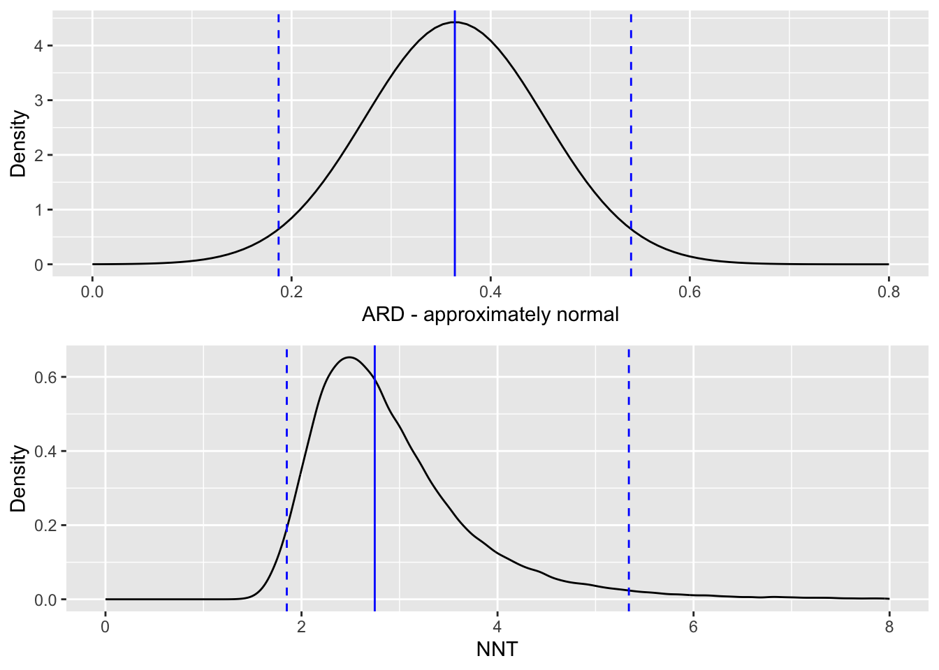
If we want to think instead in terms of NNT (the number needed to treat), then we need to find the reciprocal of our estimate of \(\tau_{ARD}\):
\[ \text{NNT} = \frac{1}{\tau_{ARD}} = \frac{1}{0.364} = 2.75.\] That is, we would expect to treat nearly three patients before one is improved (in terms of their tuberculosis symptoms). We can use the limits of the 95% CI for \(\tau_{ARD}\) to form a 95% CI for NNT, simply by taking the reciprocals of the limits to get
\[\left(\frac{1}{0.541},\; \frac{1}{0.187}\right) = \left(1.85,\; 5.33 \right).\] Because the NNT is the reciprocal of something approximately normally distributed, it has a distribution with a long tail, and we see that the confidence interval is therefore skewed.
6.2.1.2 What if the difference is not significant?
In the above section you might have already wondered what happens if the confidence interval for the absolute risk difference (ARD) contains zero. To illustrate this, we will make up some data for a small trial, loosely based on the Streptomycin data we’ve been using.
The dataset for our made-up trial is
| Successes | Failures | Total | |
|---|---|---|---|
| Treatment | 9 | 5 | 14 |
| Control | 4 | 8 | 12 |
| Total | 13 | 13 | 26 |
The ARD is now \[\frac{9}{14} - \frac{4}{12} = \frac{3}{13} \approx 0.310 \] and our 95% confidence interval for \(\tau_{ARD}\) is \(\left(-0.0567,\;0.676\right)\).
Clearly because of the small size of the trial our confidence interval is very wide (this is not a very good trial!), but the important thing to note is that it now contains zero. It looks very likely that the treatment is effective (the interval only just contains zero) but how many patients might we need to treat before we expect to see an extra success? The expected value of NNT is
\[ \frac{1}{0.310} = 3.23,\] which does not pose a problem. However, our 95% confidence interval now contains the possibility that the ARD is zero, and in this case the NNT is in some sense infinite: no matter how many patients we treat, we don’t expect to see any extra improvements. Therefore, since our confidence interval for ARD contains zero it feels appropriate that our confidence interval for NNT should contain infinity.
When thinking about a confidence interval for the NNT, we need to think about signs, and what negative and positive values mean. If both the lower and upper limits of the confidence interval for ARD are positive, there is no issue - the treatment is effective, and our NNT confidence interval is another entirely positive interval. If the confidence interval for ARD is entirely negative, we have an entirely negative interval for NNT. A negative value of NNT can be thought of as the ‘number needed to treat to harm one extra person’.
The tricky situation is when the confidence interval for the ARD is \(\left(-L, U\right)\) with \(L,U>0\), ie. an interval containing zero. As we approach zero from \(U\), the upper limit of the CI for \(\pi_T - \pi_C\), the number of patients we need to treat increases, since the treatment effect is getting smaller, until at \(\pi_T - \pi_C=0\) the NNT is infinite. Therefore, the part of the CI for NNT corresponding to the positive part of the CI for ARD is
\[\left(\frac{1}{U},\; \infty\right)\]
As we approach zero from the left in the interval (ie. from \(-L\)), the treatment gets less and less effective (and right now we mean effective in a bad way, likely doing harm to the patients compared to the control), and so we need to treat more and more patients to harm one extra patient compared to the control. In this region the NNT is negative, since if we deny some patients the treatment we will benefit a few. Therefore the CI for the NNT corresponding to the negative part of the CI for ARD is
\[\left(-\infty,\;-\frac{1}{L}\right), \] and altogether the confidence interval for the number needed to treat (NNT) is the union of these two intervals \[\left(-\infty,\;-\frac{1}{L}\right) \cup \left(\frac{1}{U},\; \infty\right).\]
The plot below shows relationship between ARD and NNT, with the intervals for our toy example shown in bold on the respective axis (the NNT interval should continue infinitely in both directions so for obvious reasons this is not all shown!).
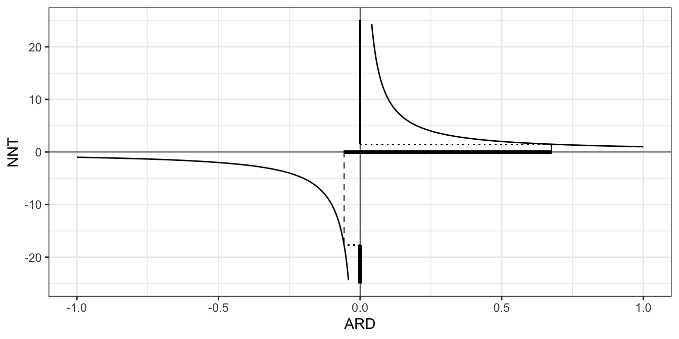
Figure 6.1: The relationship between the confidence interval for the ARD and the NNT, when the ARD interval contains zero.
Altman (1998) (available here) makes a compelling push for the use of confidence intervals for the number needed to treat. You can decide for yourself whether you agree!
Problems with the confidence interval for the ARD
You may well remember from the dim and distant past that the method we have been using so far (which in this section we’ll be calling the ‘standard’ method) is not so reliable if the proportion is close to zero or one. Newcombe (1998) compared eleven different methods for finding confidence intervals for the difference in proportions (as we are doing when we work with the ARD) and found the standard method to be the worst! The coverage probability turns out to be much lower than the nominal value, with a so-called 95% confidence interval being closer to 90% or even 85%. A further problem with this method (although it will rarely affect us in practice in this setting) is that the limits of the confidence interval aren’t forced to be in \(\left[-1,1\right]\).
We will give a sketch of the favourite method of Newcombe (1998), chosen for its ease of implementation and its accuracy, now. This is the Wilson method, first presented in Wilson (1927).
The first step is to find an interval estimate for a single proportion \(\pi\). As before, this can be written
\[\left\lbrace \pi \mid \frac{\lvert p - \pi \rvert}{\sqrt{\pi\left(1-\pi\right)/n}} \leq z_{\frac{\alpha}{2}} \right\rbrace = \left\lbrace \pi \mid \left(p - \pi\right)^2 \leq z^2_{\frac{\alpha}{2}}\frac{\pi\left(1-\pi\right)}{n} \right\rbrace. \] We can find the limits of the \(100\left(1-\alpha\right)\)% level confidence interval by changing the right hand side to an equality
\[\begin{equation} \left(p - \pi\right)^2 = z^2_{\frac{\alpha}{2}}\frac{\pi\left(1-\pi\right)}{n}. \tag{6.1} \end{equation}\]
In the standard method, we substitute \(p\) (the estimated value of \(\pi\) from our sample) into the right hand side of Equation (6.1) for \(\pi\), to get
\[\left(p - \pi\right)^2 = z^2_{\frac{\alpha}{2}}\frac{p\left(1-p\right)}{n}\]
which we solve to get the limits \[ \pi = p \pm z_{\frac{\alpha}{2}}\sqrt{\frac{p\left(1-p\right)}{n}}.\] In Wilson’s method, we instead keep \(\pi\) in the right hand side and solve the quadratic in Equation (6.1) in terms of \(\pi\).
The benefit of this new method will be most obvious for a probability that is close to 0 or 1.
Example 6.5 Suppose we have 1 success out of 50 patients, so \(p=0.02,\;n=50\).
The limits of a standard 95% confidence interval will be
\[\left(0.02 - z_{0.975}\sqrt{\frac{0.02\times{0.98}}{50}},\; 0.02 + z_{0.975}\sqrt{\frac{0.02\times{0.98}}{50}}\right) = \left(-0.0188,\;0.0588\right),\] whereas the limits to the Wilson 95% CI will be the roots of
\[\left(0.02-\pi\right)^2 = z^2_{\alpha/2}\frac{\pi\left(1-\pi\right)}{50}\] which work out to be
## [1] 0.004 0.105Visually, we can represent this as in Figure 6.2 by plotting the LHS (solid) and RHS (dashed for new method, dotted for standard method). The thick solid red line shows \(p_T\), the estimated proportion, the thinner dashed red lines show the Wilson 95% CI and the dotted red lines show the standard 95% CI. Notice that the limits of each confidence interval are formed by the points at which the solid line (LHS) crosses the dashed / dotted lines (RHS).
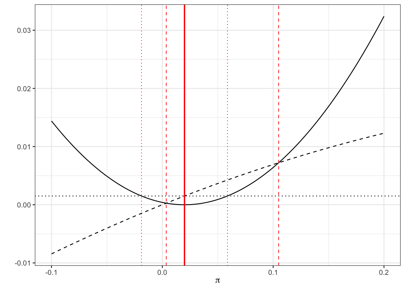
Figure 6.2: LHS of Equation 6.1 (solid black) with RHS of (black dashed) and RHS with estimate \(p\) subbed in (black dotted). The limits of the confidence intervals are where the curves cross, shown by red lines: dashed for Wilson, dotted for standard.
Example 6.6 Returning to our streptomycin example, our estimate of the probability of success for the treatment group is \(p_T = \frac{38}{55},\;n_T = 55\), and therefore our equation becomes
\[\left(\frac{38}{55} - \pi\right)^2 = z^2_{\frac{\alpha}{2}}\frac{\pi\left(1-\pi\right)}{55}.\] Solving this equation in the usual way (using the quadratic formula) we find the Wilson 95% CI to be
## [1] 0.56 0.80By contrast, in our standard method we have \[\left(\frac{38}{55} - \pi\right)^2 = z^2_{\frac{\alpha}{2}}\frac{\frac{38}{55}\left(1-\frac{38}{55}\right)}{55}\] which is
## [1] 0.57 0.81We can see this graphically
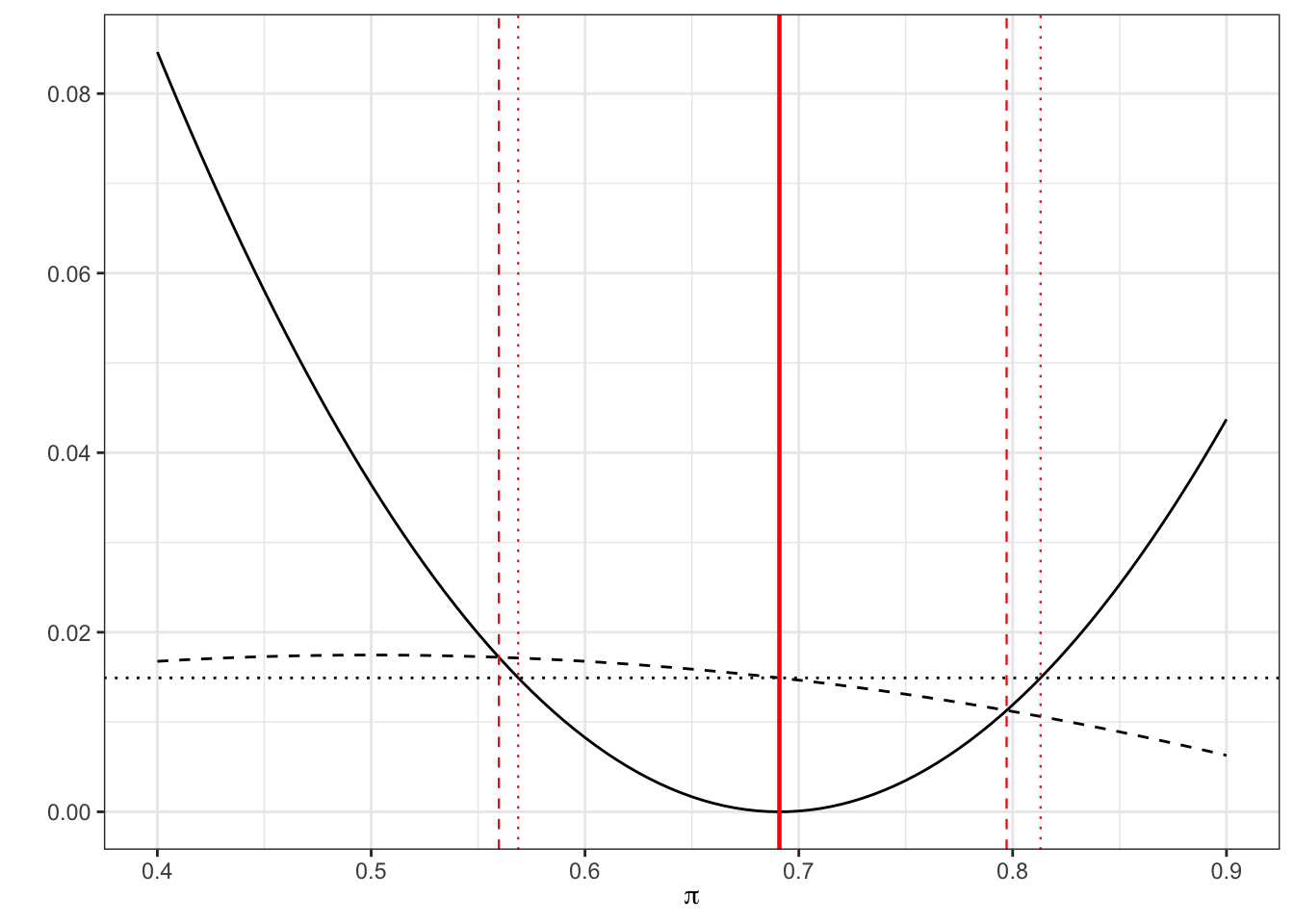
Figure 6.3: As before, dashed for Wilson, dotted for standard
Notice that the Wilson interval is asymmetric, which is more realistic.
Similarly for the control proportion \(\pi_C\), we have \(p_C = \frac{17}{52},\; n_C=52\), and our Wilson interval is
## [1] 0.22 0.46compared to the standard confidence interval
## [1] 0.20 0.45Again, we can see this graphically.
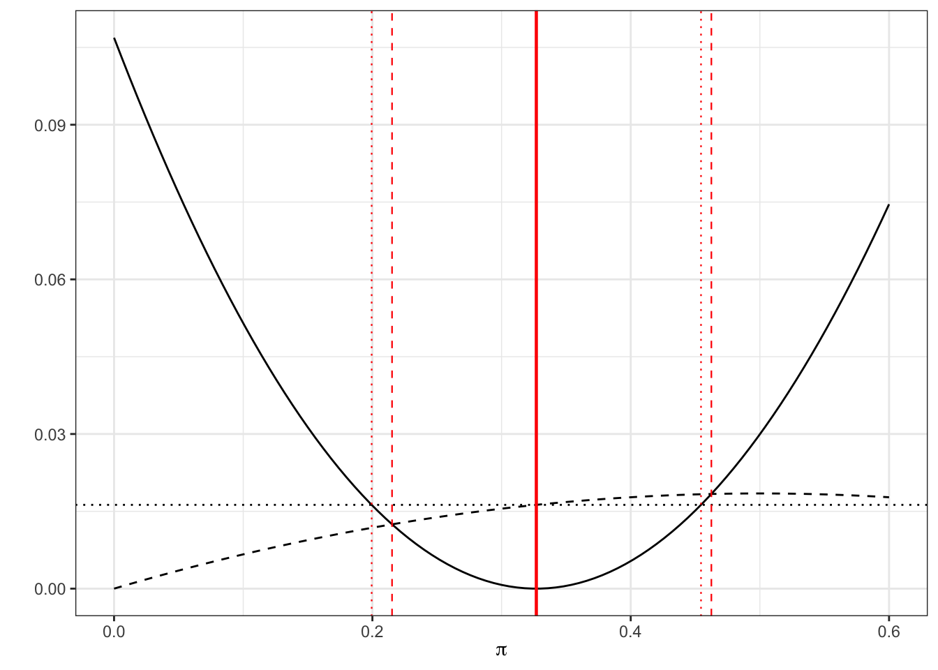
Figure 6.4: As before, dashed for Wilson, dotted for standard
6.2.1.3 Extending this to \(\pi_T - \pi_C\)
What the Wilson interval has given us is a superior method for creating confidence intervals for proportions. But, what we would like is a method for calculating a confidence interval for the difference in two proportions. You’ll be relieved to hear that there is such a method, and we’ll give a sketch here of how it works.
The limits of the ‘standard method’ confidence interval at significance level \(\alpha\) are given by
\[\begin{equation} \left(p_T - p_C - z_{\frac{\alpha}{2}}\sqrt{\frac{p_T\left(1-p_T\right)}{n_T} + \frac{p_C\left(1-p_C\right)}{n_C}},\; p_T - p_C + z_{\frac{\alpha}{2}}\sqrt{\frac{p_T\left(1-p_T\right)}{n_T} + \frac{p_C\left(1-p_C\right)}{n_C}}\right). \tag{6.2} \end{equation}\]
We can rewrite this as
\[\begin{equation} \left(p_T - p_C - \sqrt{\omega^2_T + \omega^2_C},\; p_T - p_C + \sqrt{\omega^2_T + \omega^2_C}\right) \end{equation}\]
where \(\omega_T\) and \(\omega_C\) are the widths of the separate single-sample ‘standard’ confidence intervals for \(p_T\) and \(p_C\). In Wilson’s method, we proceed in the same way, but instead use the widths of the Wilson confidence intervals for the individual probabilities \(p_T\) and \(p_C\). This is obviously a little more complicated, since the widths (eg. \(p_T - l_T\) and \(u_T - p_T\)) will now not be the same, since the Wilson CI is not symmetrical. So, we have
\[ \left(p_T - p_C - \sqrt{\left(p_T-l_T\right)^2 + \left(u_C - p_C\right)^2},\; p_T - p_C + \sqrt{\left(u_T - p_T\right)^2 + \left(p_C - l_C\right)^2}\right). \] These differences must be calculated using the individual sample confidence interval method.
Example 6.7 Applying this Wilson method to our Streptomycin example, recall that we have
\[ \begin{aligned} p_T & = \frac{38}{55}\\ p_T - l_T & = \frac{38}{55} - 0.5597 = 0.1312\\ u_T - p_T & = 0.7972 - \frac{38}{55} = 0.1064\\ p_C & = \frac{17}{52} \\ p_C - l_C & = \frac{17}{52} - 0.2152 = 0.1117\\ u_C - p_C & = 0.4624 - \frac{17}{52} = 0.1355. \end{aligned} \] Our \(95\%\) confidence interval is therefore
\[ \begin{aligned} \left(p_T - p_C - \sqrt{\left(p_T-l_T\right)^2 + \left(u_C - p_C\right)^2}\right.&,\left. p_T - p_C + \sqrt{\left(u_T - p_T\right)^2 + \left(p_C - l_C\right)^2}\right)\\ \left(\frac{38}{55}-\frac{17}{52} - \sqrt{0.1312^2 + 0.1355^2}\right.&,\left.\frac{38}{55}-\frac{17}{52} + \sqrt{0.1064^2 + 0.1117^2}\right)\\ \left(0.3640 - 0.1886 \right.&,\left. 0.3640+ 0.1543\right)\\ \left(0.157 \right.&,\left.0.500\right). \end{aligned} \] This is skewed somewhat lower than our standard CI of \(\left(0.187,\;0.541\right).\)
Returning to our earlier material, we could invert this interval to find a confidence interval for the number needed to treat (NNT).
6.2.2 Risk Ratio (RR) and Odds ratio (OR)
The measures we have looked at so far, particularly the ARD, are quite analagous to the continuous normally distributed case. However, there are yet more commonly used measures of difference for proportions, which need to be dealt with differently, but also afford more opportunities for modelling.
The risk ratio is defined as
\[\text{RR} = \frac{\pi_T}{\pi_C}\]
The odds ratio is defined as \[\text{OR} = \frac{\pi_T/\left(1-\pi_T\right)}{\pi_C/\left(1-\pi_C\right)}\] The first thing to note is that for both the risk ratio and the odds ratio, the null value is one (not zero, as for the ARD), and both values must always be positive. We think about things multiplicatively, so for example if \(RR=3\) we can say that the event is “3 times more likely” in group \(T\) than in group \(C\).
Odds
Odds and odds ratios are a bit trickier to think about (this article explains them really well - it’s aimed at ‘kids and teens’ but don’t let that put you off!). The odds of an event are the probability of it happening over the probability of it not happening. So, if (for some event \(A\)), \(p\left(A\right)=0.2\), the odds of \(A\) are
\[\frac{p\left(A\right)}{p\left(A'\right)} = \frac{0.2}{0.8} = \frac{1}{4}, \] which we say as “1 to 4” or 1:4. For every one time \(A\) occurs, we expect it not to occur four times.
The odds ratio compares the odds of the outcome of interest in the Treament group with the odds of that event in the Control group. It tells us how the odds of the event are affected by the treatment (vs control).
With the ARD, if we compare treatments in one direction (say \(p_T - p_C\)) we would obtain the negative of the interval for the other way (\(p_C - p_T\)). With the RR and OR, the discrepancy between two proportions is given by a ratio, and so comparing them in one direction (\(p_T / p_C\)) will give the reciprocal of the other direction (\(p_C / p_T\)).
Example 6.8 For our Streptomycin example, we estimated the ARD by \[\hat\tau_{ARD}=p_T - p_C = \frac{38}{55} - \frac{17}{52} = 0.364,\] or could have alternatively had \[\hat\tau_{ARD}=p_C - p_T = \frac{17}{52} - \frac{38}{55} = - 0.364.\] For the risk ratio, we have
\[\hat{\tau}_{RR} = \frac{p_T}{p_C} = \frac{38/55}{17/52} = 2.113,\] or could alternatively have
\[\hat{\tau}_{RR} = \frac{p_C}{p_T} = \frac{17/52}{38/55} = 0.473 = \frac{1}{2.113}.\] We could say that a patient is “more than twice as likely to be cured with streptomycin than by the control”.
For the odds ratio, we have
\[\hat{\tau}_{OR} = \frac{p_T/\left(1-p_T\right)}{p_C/\left(1-p_C\right)} = \frac{(38/55)/(17/55)}{(17/52)/(35/52)} = 4.602, \] and therefore the odds of recovery are around 4.6 greater for Streptomycin than for the control. Similarly, we could reframe this as
\[\hat{\tau}_{OR} = \frac{p_C/\left(1-p_C\right)}{p_T/\left(1-p_T\right)} = \frac{(17/52)/(35/52)}{(38/55)/(17/55)} = 0.217 = \frac{1}{4.602}.\]
6.2.2.1 Confidence intervals for RR and OR
One thing to notice is that symmetry works differently on the RR and OR scale from on the ARD scale. There is an equivalence between an interval \(\left(l,\,u\right)\) (with \(l,u>1\)) and \(\left(\frac{1}{u},\frac{1}{l}\right)\), since these intervals would equate to comparing the same two treatments in different directions (assuming the difference was significant and neither interval contains 1). Similarly, on this scale the interval
\[\left(\frac{1}{k},\,k\right) \text{ for some }k>1 \] can be thought of as symmetric, in that one treatment may be up to \(k\) times more effective than the other, in either direction. Therefore, to build a confidence interval for OR or RR, we will not be following the usual formula
\[\text{point estimate } \pm{z\times{SE}}.\] You may have already been thinking that a log transformation would be useful here, and you’d be correct! The sort-of symmetric intervals we’ve been discussing here actually are symmetric (about zero) on the log scale.
Firstly we’ll consider the risk ratio. Let’s define
\[ \phi = \log\left(\frac{\pi_T}{\pi_C}\right).\] The natural way to estimate this is with the sample proportions
\[\log\left(\frac{p_T}{p_C}\right) = \log\left(p_T\right) - \log\left(p_C\right).\] These estimated proportions should be approximately normal and independent of one another, and so \(\log\left(\frac{p_T}{p_C}\right)\) is approximately normal with mean \(\phi\) (the true value) and variance
\[\operatorname{var}\left(\log\left(p_T\right)\right) + \operatorname{var}\left(\log\left(p_C\right)\right). \] We can now apply the Delta method (see section 5.1) to find that (using Equation (5.3))
\[\operatorname{var}\left[\log\left(p_T\right)\right] = \operatorname{var}\left[\log\left(\frac{r_T}{n_T}\right)\right] \approx \frac{\pi_T\left(1-\pi_T\right)}{n_T}\times{\left(\frac{1}{\pi_T}\right)^2} = \frac{1}{n_T\pi_T} - \frac{1}{n_T}. \] Since we estimate \(\pi_T\) by \(r_T/n_T\) this can be estimated by \(r_T^{-1} - n_T^{-1}\). Notice that we are relying on the derivative of \(\log\left(x\right)\) being \(x^{-1}\), so we must always use natural logarithms.
This leads us to the result that, approximately
\[\log\left(\frac{p_T}{p_C}\right) \sim N\bigg(\phi,\,\left(r_T^{-1} - n_T^{-1}\right) + \left(r_C^{-1} - n_C^{-1}\right) \bigg) \] and so we can generate \(100\left(1-\alpha\right)\)% confidence intervals for \(\phi\) as \(\left(l_{RR},\;u_{RR}\right)\), where the limits are
\[ \log\left(\frac{p_T}{p_C}\right) \pm z_{\frac{\alpha}{2}}\sqrt{\left(r_T^{-1} - n_T^{-1}\right) + \left(r_C^{-1} - n_C^{-1}\right)}. \] This then translates to an interval for the risk ratio itself of \(\left(e^{l_{RR}},e^{u_{RR}}\right)\).
Example 6.9 Returning once again to our streptomycin example, recall that we have
\[ \begin{aligned} r_T & = 38\\ n_T & = 55 \\ r_C & = 17 \\ n_C & = 52 \end{aligned} \] and so the limits of the confidence interval (with \(\alpha=0.05\)) on the log scale are
\[\log\left(\frac{38/55}{17/52}\right) \pm 1.96\sqrt{\left(\frac{1}{38} - \frac{1}{55}\right) + \left(\frac{1}{17} - \frac{1}{52}\right)} = \log(2.11) \pm 1.96 \times 0.218\]
which gives us \(\left(0.320,\,1.176\right)\) on the log scale, and a 95% CI for the risk ratio of \(\left(1.377,\,3.243\right)\).
So, we’ve seen that we can find confidence intervals for each of our four measures of difference. But we probably want to also be able to incorporate baseline measurements, as we did for continuous outcome variables.
6.3 Accounting for baseline observations: logistic regression
We saw with the continuous outcomes that it is often advantageous to include baseline measurements of the outcome (if they are known) in our analysis, and this is no less true for binary outcomes.
In this section we use the term ‘baseline observations’ to mean any measurement that was known before the trial started. Unlike with continuous measurements, with a binary outcome, there is not usually a pre-trial value of the primary outcome. A binary outcome is often already relative to pre-trial (for example ‘Have the patient’s symptoms improved?’) or refers to an event that definitely wouldn’t have happened pre-trial (for example ‘Did the patient die within the next 6 months?’ or ‘Was the patient cured?’). However, as we saw with ANCOVA, we can include other sorts of covariates in a linear model, so this is fine.
The general form of model that we would like for patient \(i\) is
\[\text{outcome}_i = \mu + \tau G_i + \beta_1\times{\text{baseline}_{1i}} + \ldots + \beta_p\times{\text{baseline}_{pi}} + \text{error}_i,\] where \(G_i\) is an indicator function taking values 1 if patient \(i\) was in group \(T\) and 0 if they were in group \(C\), and \(\text{baseline}_1,\;\ldots,\;\text{baseline}_p\) are \(p\) baseline measurements that we would like to take into account.
However, this actually creates quite a few problems with binary variables. The outcome for patient \(i\) will be either 0 or 1, but the terms in the model above do not guarantee this at all. Adding a normally distributed error term doesn’t really make sense in this context, so we will remove it. We can also make the LHS more continuous by thinking of the mean outcome rather than a single outcome. This makes sense, since if several patients were identical to patient \(i\) (in the sense of having the same baseline covariate values and being allocated to the same treatment), we probably wouldn’t expect them all to have exactly the same outcome. Therefore we might instead think in terms of mean outcome, in which case our model becomes
\[\text{mean outcome}_i = \mu + \tau G_i + \beta_1\times{\text{baseline}_{1i}} + \ldots + \beta_p\times{\text{baseline}_{pi}}.\]
There is one final problem to overcome, which is that the LHS will certainly be in \(\left[0,\;1\right]\), but the RHS could take any value. To address this we need to use a transformation, to take the mean outcome from \(\left[0,1\right]\) to \(\mathbb{R}\).
The transformation that is usually used for a binary variable is the logit function, which is the log of the odds,
\[\operatorname{logit}\left(\pi\right) = \log\frac{\pi}{1-\pi}.\]
As \(\pi\) tends to zero, \(\operatorname{logit}\left(\pi\right)\) tends to \(-\infty\), and as \(\pi\) tends to one, \(\operatorname{logit}\left(\pi\right)\) tends to \(\infty\). The derivative of the \(\operatorname{logit}\) function is
\[ \frac{d\operatorname{logit}\left(\pi\right)}{d\pi} = \frac{1}{\pi\left(1-\pi\right)}\] which is always positive for \(\pi\in\left[0,1\right]\). This means that we can use it to transform our mean outcome (which we will now call \(\pi\), since the mean outcome is the estimate of the probability of success) in the model
\[\begin{equation} \operatorname{logit}\left(\pi\right) = \mu + \tau G + \beta_1\times{\text{baseline}_{1}} + \ldots + \beta_p\times{\text{baseline}_{p}} \tag{6.3} \end{equation}\]
and any value in \(\mathbb{R}\) is allowed on both sides. This model is known as logistic regression, and belongs to a class of models called Generalized Linear Models. If you did Advanced Statistical Modelling III you’ll have seen these before. If you haven’t seen them, and want to know more, this article gives a nice introduction (and some useful R tips!).
6.3.1 What does this model tell us?
We now have an equation for a model that makes sense, but what is it actually modelling? And what does it tell us about the effect of the treatment? Consider the difference between two patients who are the same in every respect except one is assigned to group \(C\) (so \(G=0\)) and the other to group \(T\) (so \(G=1\)). The model gives:
\[ \begin{aligned} \operatorname{logit}\left(\pi\right) = \log\left(\frac{\pi}{1-\pi}\right) = \log\left(\text{Odds of success}\right) & = \mu + \tau + \beta_1x_1 + \ldots + \beta_px_p & \text{ (group T)}\\ \operatorname{logit}\left(\pi\right) = \log\left(\frac{\pi}{1-\pi}\right) = \log\left(\text{Odds of success}\right) & = \mu + \beta_1x_1 + \ldots + \beta_px_p & \text{ (group C)} \end{aligned} \] Subtracting one from the other, we find
\[ \begin{aligned} \log(\text{Odds of success for group T}) - & \log(\text{Odds of success for group C})\\ &= \log\left(\frac{\text{Odds of success for group T}}{\text{Odds of success for group C}}\right) = \log\left(OR\right) \\ &= \tau. \end{aligned} \]
That is, \(\tau\) is the log of the odds ratio, or \(e^\tau\) is the odds ratio adjusted for variables \(x_1,\;\ldots,\;x_p\). Put another way, while the baseline covariates \(x_1,\ldots,x_p\) affect the probability of ‘success’ (or whatever our binary outcome’s one means), \(\tau\) is a measure of the effect of the treatment compared to control given some set of baseline covariate values.
6.3.2 Fitting a logistic regression model
Logistic regression models are generally fitted using maximum likelihood. In the notation of Equation (6.3), the parameters we need to fit are the coefficients \(\mu,\;\tau\) and \(\beta_1,\ldots,\beta_p\). To ease notation for this section we will collect these into a vector \(\boldsymbol\beta\), with \(\beta_0=\mu\) and \(\beta_{p+1}=\tau\), so that our \(G\) variable is now \(x_{p+1}\).
This notation allows us to write the linear function on the RHS of Equation (6.3) for participant \(i\) as
\[x_i^T\boldsymbol\beta = \sum\limits_{j=0}^{p+2} x_{ij}\beta_j, \] where
- \(x_{i0}=1\) (so that \(\beta_0\) is the intercept \(\mu\))
- \(x_{i1},\ldots,x_{ip}\) are the baseline covariates.
- \(x_{i,p+1}= \begin{cases} 0\text{ if participant }i\text{ is in group }C\\ 1\text{ if participant }i\text{ is in group }T \end{cases}\)
If \(\pi_i\) is the probability that the outcome for participant \(i\) is 1, where \(i=1,\ldots,n\), then the logistic model specifies these \(n\) parameters through the \(p+2\) parameters \(\beta_j\), via the \(n\) expressions
\[\begin{equation} \operatorname{logit}\left(\pi_i\right) = x_i^T\boldsymbol\beta. \tag{6.4} \end{equation}\]
Using the Bernoulli distribution, the log-likelihood given data \(y_1,\ldots,y_n\) is
\[\begin{align*} \ell\left(\left\lbrace\pi_i \right\rbrace \mid\left\lbrace y_i\right\rbrace\right) & = \sum\limits_{i=1}^n\left[y_i\log(\pi_i) + \left(1-y_i\right)\log\left(1-\pi_i\right)\right]\\ & = \sum\limits_{i=1}^n\left[y_i\log\left(\frac{\pi_i}{1-\pi_i}\right) + \log\left(1-\pi_i\right)\right], \end{align*}\] where \(y_i=0\) or 1 is the outcome for participant \(i\). Using Equation (6.4) we can rewrite this in terms of \(\boldsymbol\beta\) as
\[\ell\left(\left\lbrace\beta_j \right\rbrace\mid{\text{data}}\right) = \sum\limits_{i=1}^n \left[y_i x_i^T\boldsymbol\beta - \log\left(1+e^{x_i^T\boldsymbol\beta}\right)\right].\]
The fitted model is then the one with the values \(\beta_j\), \(j=0,\dots,q\), that maximise this expression (and hence maximise the likelihood itself), which we will label the \(\left\lbrace \hat{\beta}_j\right\rbrace\).
This is generally done some via some numerical method, and we won’t go into that here. The method used by R will generate the MLE \(\hat\beta_j\) for each \(\beta_j\), and also an estimate of the standard error of each \(\hat\beta_j\). In particular there will be an estimate of the standard error of \(\hat\beta_1\), better known as \(\hat\tau\), the estimate of the treatment effect. This is important, because it means we can test the hypothesis that \(\tau=0\), and can form a confidence interval for the adjusted log odds ratio.
Example 6.10 This study is detailed in Elmunzer et al. (2012). ERCP, or endoscopic retrograde cholangio-pancreatogram, is a procedure performed by threading an endoscope through the mouth to the opening in the duodenum where bile and pancreatic digestive juices are released into the intestine. ERCP is helpful for treating blockages of flow of bile (gallstones, cancer), or diagnosing cancers of the pancreas, but has a high rate of complications (15-25%). The occurrence of post-ERCP pancreatitis is a common and feared complication, as pancreatitis can result in multisystem organ failure and death, and can occur in ~ 16% of ERCP procedures. This study tests whether the use of anti-inflammatory NSAID therapies at the time of ERCP reduce the rate of this complication. The study had 602 participants.
The dataset contains 33 variables, but we will focus on a small number:
- \(X\): (primary outcome) - incidence of post-ercp pancreatitis 0 (no), 1 (yes).
- Treatment arm
rx: 0 (placebo), 1 (treatment) - Site: 1, 2, 3, 4
- Risk: Risk score (1 to 5). Should be factor but treated as continuous.
- Age: from 19 to 90, mean 45.27, SD 13.30.
The correlation between risk and age is -0.216, suggesting no problems of collinearity between those two variables.
Note: an obvious one to include would be gender, but I tried it and it is not at all significant, so I have pre-whittled it down for [even more] simplicity.
##        id           site          age             risk        outcome                 rx
##  Min.   :1001   1_UM  :164   Min.   :19.00   Min.   :1.000   0_no :523   0_placebo     :307
##  1st Qu.:1152   2_IU  :413   1st Qu.:35.00   1st Qu.:1.500   1_yes: 79   1_indomethacin:295
##  Median :2138   3_UK  : 22   Median :45.00   Median :2.500
##  Mean   :1939   4_Case:  3   Mean   :45.27   Mean   :2.381
##  3rd Qu.:2289                3rd Qu.:54.00   3rd Qu.:3.000
##  Max.   :4003                Max.   :90.00   Max.   :5.500
## Some things to note:
# There are very few patients from site 4, and not many from site 3
# The age range goes from 19 to 90
# 'rx' is the group variable
## We will try models with age and age^2
glm_indo_agelin = glm(outcome ~ age + site + risk + rx, data=indo_rct,
family = binomial(link = "logit"))
glm_indo_agesq = glm(outcome ~ I(age^2) + site + risk + rx, data=indo_rct,
family = binomial(link = "logit"))
print(summary(glm_indo_agelin), digits=2)##
## Call:
## glm(formula = outcome ~ age + site + risk + rx, family = binomial(link = "logit"),
## data = indo_rct)
##
## Coefficients:
## Estimate Std. Error z value Pr(>|z|)
## (Intercept) -1.7863 0.6414 -2.8 0.005 **
## age -0.0085 0.0099 -0.9 0.394
## site2_IU -1.2293 0.2693 -4.6 5e-06 ***
## site3_UK -1.1279 0.7759 -1.5 0.146
## site4_Case -13.8644 827.9211 0.0 0.987
## risk 0.5619 0.1423 3.9 8e-05 ***
## rx1_indomethacin -0.7633 0.2615 -2.9 0.004 **
## ---
## Signif. codes: 0 '***' 0.001 '**' 0.01 '*' 0.05 '.' 0.1 ' ' 1
##
## (Dispersion parameter for binomial family taken to be 1)
##
## Null deviance: 468.01 on 601 degrees of freedom
## Residual deviance: 427.07 on 595 degrees of freedom
## AIC: 441.1
##
## Number of Fisher Scoring iterations: 14## GVIF Df GVIF^(1/(2*Df))
## age 1.046789 1 1.023127
## site 1.089701 3 1.014420
## risk 1.127145 1 1.061671
## rx 1.008980 1 1.004480##
## Call:
## glm(formula = outcome ~ I(age^2) + site + risk + rx, family = binomial(link = "logit"),
## data = indo_rct)
##
## Coefficients:
## Estimate Std. Error z value Pr(>|z|)
## (Intercept) -2.0e+00 4.9e-01 -4.0 7e-05 ***
## I(age^2) -9.4e-05 1.1e-04 -0.9 0.385
## site2_IU -1.2e+00 2.7e-01 -4.6 5e-06 ***
## site3_UK -1.1e+00 7.8e-01 -1.5 0.144
## site4_Case -1.4e+01 8.3e+02 0.0 0.987
## risk 5.6e-01 1.4e-01 3.9 9e-05 ***
## rx1_indomethacin -7.6e-01 2.6e-01 -2.9 0.004 **
## ---
## Signif. codes: 0 '***' 0.001 '**' 0.01 '*' 0.05 '.' 0.1 ' ' 1
##
## (Dispersion parameter for binomial family taken to be 1)
##
## Null deviance: 468.01 on 601 degrees of freedom
## Residual deviance: 427.03 on 595 degrees of freedom
## AIC: 441
##
## Number of Fisher Scoring iterations: 14## GVIF Df GVIF^(1/(2*Df))
## I(age^2) 1.052813 1 1.026067
## site 1.089772 3 1.014431
## risk 1.132658 1 1.064264
## rx 1.007972 1 1.003978Since neither age nor age^2 appear influential, and the AIC and residual deviance values are almost identical, we’ll remove it and keep the other covariates.
glm_indo = glm(outcome ~ site + risk + rx, data=indo_rct, family = binomial(link = "logit"))
print(summary(glm_indo), digits=2)
##
## Call:
## glm(formula = outcome ~ site + risk + rx, family = binomial(link = "logit"),
## data = indo_rct)
##
## Coefficients:
## Estimate Std. Error z value Pr(>|z|)
## (Intercept) -2.23 0.38 -5.8 5e-09 ***
## site2_IU -1.22 0.27 -4.5 6e-06 ***
## site3_UK -1.13 0.78 -1.5 0.145
## site4_Case -13.84 833.24 0.0 0.987
## risk 0.58 0.14 4.2 3e-05 ***
## rx1_indomethacin -0.75 0.26 -2.9 0.004 **
## ---
## Signif. codes: 0 '***' 0.001 '**' 0.01 '*' 0.05 '.' 0.1 ' ' 1
##
## (Dispersion parameter for binomial family taken to be 1)
##
## Null deviance: 468.01 on 601 degrees of freedom
## Residual deviance: 427.81 on 596 degrees of freedom
## AIC: 439.8
##
## Number of Fisher Scoring iterations: 14## GVIF Df GVIF^(1/(2*Df))
## site 1.088963 3 1.014306
## risk 1.094106 1 1.045995
## rx 1.005852 1 1.002922Notice that
- The estimate and standard error of \(\hat{\tau}\) (the coefficient of
rx) haven’t changed much at all (mainly because, as the VIF shows us, there are no issues with multicollinearity) - The standard error for the site 4 cases is enormous - this is because there are so few observations.
From the summary we see that \(\hat\tau = -0.752\), with a standard error of 0.261. A 95% CI for \(\tau\) is therefore
\[-0.752 \pm 1.96\times 0.261 = \left(-1.26,\;-0.240\right).\] Recall that \(\tau\) is the log of the odd ratio, so we can make this (slightly) more intuitive by finding a confidence interval for the odds ratio itself:
\[\left(\exp(-1.26),\;\exp(-0.240)\right) = \left(0.28,\,0.79\right).\]
This model supports the hypothesis that the log of the odds ratio isn’t zero, and therefore we can reject \(H_0\).
We can also use the model to estimate the odds of ‘success’ (the outcome 1) for different groups of patients, by fixing the values of the covariates. The linear expression \(x^T\hat{\boldsymbol\beta}\) for given values of \(x\) gives us as estimate of
\[\log\left(\frac{p(X=1)}{1-p(X=1)}\right),\] where \(X\) here is the primary outcome. The exponent of this therefore gives the odds, and this can be rearranged to find the probability,
\[p\left(X_i=1\right) = \frac{\exp(\text{logit}_i)}{1+\exp(\text{logit}_i)}, \] where \(\text{logit}_i\) is the fitted value of the linear model (on the logit scale) given all the baseline characteristics of some patient \(i\). This will be the probability, according to the model, that a patient with this particular combination of baseline characteristics will have outcome 1.
Example 6.11 Continuing with Example 6.10, we can find estimates of the log odds (and therefore the odds) of post-ECRP pancreatitis for various categories of patient.
For this we will make use of the summary table
##
## Call:
## glm(formula = outcome ~ site + risk + rx, family = binomial(link = "logit"),
##     data = indo_rct)
##
## Coefficients:
##                  Estimate Std. Error z value Pr(>|z|)
## (Intercept)         -2.23       0.38    -5.8    5e-09 ***
## site2_IU            -1.22       0.27    -4.5    6e-06 ***
## site3_UK            -1.13       0.78    -1.5    0.145
## site4_Case         -13.84     833.24     0.0    0.987
## risk                 0.58       0.14     4.2    3e-05 ***
## rx1_indomethacin    -0.75       0.26    -2.9    0.004 **
## ---
## Signif. codes:  0 '***' 0.001 '**' 0.01 '*' 0.05 '.' 0.1 ' ' 1
##
## (Dispersion parameter for binomial family taken to be 1)
##
##     Null deviance: 468.01  on 601  degrees of freedom
## Residual deviance: 427.81  on 596  degrees of freedom
## AIC: 439.8
##
## Number of Fisher Scoring iterations: 14For example, a patient from site 1, with risk level 3, in the control group would have odds
\[\exp\left(-2.2307 + 3\times 0.5846\right) = 0.6207, \] which translates to a probability of post-ECRP pancreatitis of
\[\frac{0.6207}{1+0.6207} = 0.383. \]
By contrast, a patient in group \(T\), from site 2, at risk level 1, would have odds
\[\exp\left(-2.2307 - 1.2204 + 1\times 0.5846 - 0.7523\right) = 0.0268, \] which is equivalent to a probability of post-ECRP pancreatitis of
\[\frac{0.0268}{1+0.0268} = 0.0261.\]
Being more methodical we can collect these into a table, and use predict.glm. This also has the advantage that we can find the standard error for the log odds ratio for each category. Since the site 3 and 4 coefficents are not significant (mainly due to a lack of data), we will focus only on the site 1 and 2 participants.
## Create data frame with every combination of factors (only showing sites 1 and 2)
df_indo = data.frame(
  site = rep(c(rep("2_IU", 5), rep("1_UM", 5)),2),
  risk = rep(1:5, 4),
  rx = rep(c("0_placebo", "1_indomethacin"), c(10,10))
)

## Find and transform fitted value

df_indo$logodds = predict(glm_indo, newdata=df_indo, se.fit = T)$fit
df_indo$logodds_se = predict(glm_indo, newdata=df_indo, se.fit = T)$se.fit
df_indo$logor_lower = df_indo$logodds - qnorm(0.975)*df_indo$logodds_se
df_indo$logor_upper = df_indo$logodds + qnorm(0.975)*df_indo$logodds_se

df_indo$odds = exp(df_indo$logodds)
df_indo$odds_lower = exp(df_indo$logor_lower)
df_indo$odds_upper = exp(df_indo$logor_upper)

df_indo$prob_lower = df_indo$odds_lower/(1+df_indo$odds_lower)
df_indo$prob = df_indo$odds/(1+df_indo$odds)
df_indo$prob_upper = df_indo$odds_upper/(1+df_indo$odds_upper)


df_indo_round2 <- df_indo %>%                   # Using dplyr functions
  mutate_if(is.numeric,
            round,
            digits = 2)
df_indo_round2 |>
  kable() |>
kable_styling("striped")| site | risk | rx | logodds | logodds_se | logor_lower | logor_upper | odds | odds_lower | odds_upper | prob_lower | prob | prob_upper |
|---|---|---|---|---|---|---|---|---|---|---|---|---|
| 2_IU | 1 | 0_placebo | -2.87 | 0.32 | -3.48 | -2.25 | 0.06 | 0.03 | 0.11 | 0.03 | 0.05 | 0.10 |
| 2_IU | 2 | 0_placebo | -2.28 | 0.22 | -2.72 | -1.85 | 0.10 | 0.07 | 0.16 | 0.06 | 0.09 | 0.14 |
| 2_IU | 3 | 0_placebo | -1.70 | 0.19 | -2.08 | -1.32 | 0.18 | 0.13 | 0.27 | 0.11 | 0.15 | 0.21 |
| 2_IU | 4 | 0_placebo | -1.11 | 0.26 | -1.61 | -0.61 | 0.33 | 0.20 | 0.54 | 0.17 | 0.25 | 0.35 |
| 2_IU | 5 | 0_placebo | -0.53 | 0.36 | -1.24 | 0.18 | 0.59 | 0.29 | 1.20 | 0.22 | 0.37 | 0.55 |
| 1_UM | 1 | 0_placebo | -1.65 | 0.28 | -2.19 | -1.10 | 0.19 | 0.11 | 0.33 | 0.10 | 0.16 | 0.25 |
| 1_UM | 2 | 0_placebo | -1.06 | 0.22 | -1.49 | -0.63 | 0.35 | 0.22 | 0.53 | 0.18 | 0.26 | 0.35 |
| 1_UM | 3 | 0_placebo | -0.48 | 0.24 | -0.95 | 0.00 | 0.62 | 0.39 | 1.00 | 0.28 | 0.38 | 0.50 |
| 1_UM | 4 | 0_placebo | 0.11 | 0.33 | -0.54 | 0.75 | 1.11 | 0.59 | 2.12 | 0.37 | 0.53 | 0.68 |
| 1_UM | 5 | 0_placebo | 0.69 | 0.44 | -0.17 | 1.56 | 2.00 | 0.84 | 4.76 | 0.46 | 0.67 | 0.83 |
| 2_IU | 1 | 1_indomethacin | -3.62 | 0.36 | -4.32 | -2.92 | 0.03 | 0.01 | 0.05 | 0.01 | 0.03 | 0.05 |
| 2_IU | 2 | 1_indomethacin | -3.03 | 0.27 | -3.56 | -2.51 | 0.05 | 0.03 | 0.08 | 0.03 | 0.05 | 0.08 |
| 2_IU | 3 | 1_indomethacin | -2.45 | 0.24 | -2.91 | -1.99 | 0.09 | 0.05 | 0.14 | 0.05 | 0.08 | 0.12 |
| 2_IU | 4 | 1_indomethacin | -1.86 | 0.28 | -2.41 | -1.32 | 0.15 | 0.09 | 0.27 | 0.08 | 0.13 | 0.21 |
| 2_IU | 5 | 1_indomethacin | -1.28 | 0.37 | -2.01 | -0.55 | 0.28 | 0.13 | 0.58 | 0.12 | 0.22 | 0.37 |
| 1_UM | 1 | 1_indomethacin | -2.40 | 0.32 | -3.02 | -1.77 | 0.09 | 0.05 | 0.17 | 0.05 | 0.08 | 0.15 |
| 1_UM | 2 | 1_indomethacin | -1.81 | 0.26 | -2.32 | -1.30 | 0.16 | 0.10 | 0.27 | 0.09 | 0.14 | 0.21 |
| 1_UM | 3 | 1_indomethacin | -1.23 | 0.27 | -1.76 | -0.70 | 0.29 | 0.17 | 0.50 | 0.15 | 0.23 | 0.33 |
| 1_UM | 4 | 1_indomethacin | -0.64 | 0.34 | -1.31 | 0.02 | 0.52 | 0.27 | 1.02 | 0.21 | 0.34 | 0.51 |
| 1_UM | 5 | 1_indomethacin | -0.06 | 0.45 | -0.93 | 0.81 | 0.94 | 0.39 | 2.25 | 0.28 | 0.49 | 0.69 |
6.4 Diagnostics for logistic regression
There are many diagnostic techniques for binomial data (see eg. Collett (2003a)) but we will only touch on a small number. Unlike with a linear regression model, we don’t have residuals to analyse, because our model output is fundamentally different from our data: our model outputs are probabilities, but our data is all either 0 or 1. Just because a particular patient had an outcome of 1, we can’t conclude that their probability should have been high. If the ‘true’ probability of \(X=1\) for some group of similar (in the baseline covariates sense) patients is 0.9, this means we should expect 1 in 10 of these patients to have \(X=0\).
This makes assessing logistic regression models somewhat tricky.
Diagnostics for logistic regression fall into two categories: discrimination and calibration. We will look at each of these in turn, though by no means exhaustively.
6.4.1 Discrimination
Here we are thinking of the logistic regression model as a classifier: for each participant the model outputs some value, on the \(\operatorname{logit}\left(p\right)\) scale. If that value is below some threshold, we classify that participant as 0. If the value is above the threshold, we classify them as 1. We are slightly abandoning the notion that the model is predicting probabilities, and instead testing whether the model can successfully order the patients correctly. Can we set some threshold on the model output that (almost) separates the cohort into its ones and zeros?
A classic way to asses this is by using Receiver Operating Characteric (ROC) analysis. ROC analysis was developed during the second world war, as radar operators analysed their classification accuracy in distinguishing signal (eg. an enemy plane) from noise. It is still widely used in the field of statistical classification, including in medical diagnostics. ROC analysis can be applied to any binary classifier, not just logistic regression.
6.4.1.1 ROC analysis
To understand ROC analysis, we need to revisit two concepts relating to tests or classifiers that you might not have seen since Stats I, and we will introduce (or remind ourselves of) some notation to do this:
- \(\hat{p}_i\in\left(0,1\right)\) is the fitted value of the logistic regression model for patient \(i\)
- \(X_i=0\) or \(1\) is the true outcome for patient \(i\)
- \(t\in\left(0,1\right)\) is the threshold value.
If \(\hat{p}_i<t\) we classify patient \(i\) as 0, if \(\hat{p}\geq t\) we classify them as 1. The language of ROC analysis is so entrenched in diagnostic/screening tests that I have kept it here for consistency. A ‘positive’ result for us is \(X=1\), and a ‘negative’ result is \(X=0\).
Definition 6.1 The sensitivity of a test (or classifier) is the probability that it will output positive (or 1) if the true value is positive (or 1): \[p\left(\hat{p}_i \geq t \mid{X_i=1}\right).\]
Definition 6.2 The specificity of a test (or classifier) is the probability that it will output negative (or 0) if the true value is negative (or 0):
\[p\left(\hat{p}_i < t \mid{X_i=0}\right) \]
We estimate these by the proportions within the dataset.
These are very commonly used for thinking about diagnostic tests and screening tests, and in these contexts a ‘success’ or ‘positive’ is almost always the presence of some condition or disease. In our context, we need to be mindful that a 1 could be good or bad, depending on the trial.
The core part of a ROC analysis is to plot sensitivity against 1-specificity for every possible value of the threshold. In a logistic regression context, the lowest the threshold can be is zero. If we set the \(t=0\), the model will predict everyone to have an outcome of 1. The sensitivity will be 1 and the specificity will be 0. At the other extreme, if we set \(t=1\), we will classify everyone as a 0, and have sensitivity 0 and specificity 1. If we vary the threshold from 0 to 1 the number of people classified in each group will change, and so will the sensitivity and specificity. This forms a ROC curve.
The plots below shows the distributions of fitted values for patients with \(X=0\) and \(X=1\), for models with good and poor separation, and the corresponding ROC curves. The threshold is (arbitrarily) set to 0.5, and so the Sensitivity and Specificity reflect that. The AUC (area under the curve) is an overall summary of the model’s predictive efficacy. If AUC=1, the model is perfect. If AUC is 0.5, the model is no better than random guessing. Generally it is thought that AUC around 0.8 is quite good, and AUC around 0.9 is excellent.
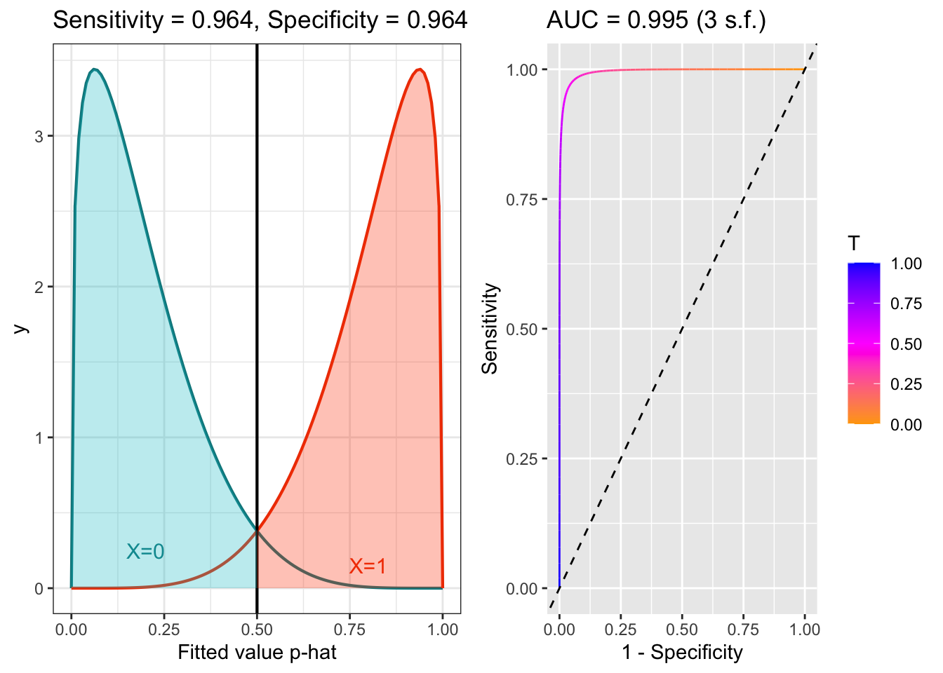
Figure 6.5: ROC example with good separation.
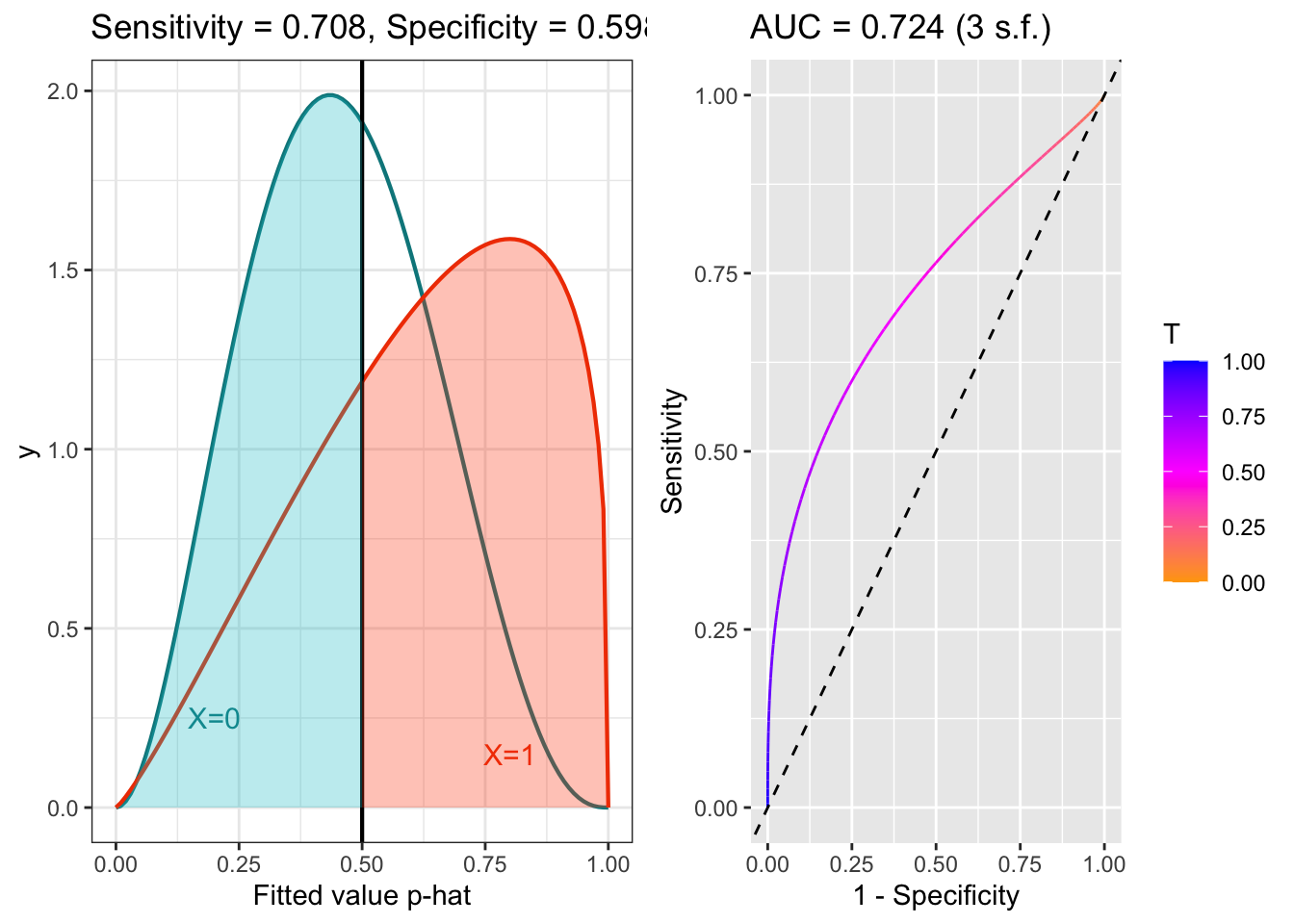
Figure 6.6: ROC example with poor separation.
Note that I’ve used beta distributions for some hypothetical distributions of fitted values for the different groups, but this is just for convenience: ROC analysis makes no distributional assumptions.
Example 6.12 Let’s look at the model we fitted in Example 6.10. To draw the ROC curve of this data, we will use the R package pROC.
fit_indo = fitted(glm_indo)   # Fitted values from glm_indo
out_indo = indo_rct$outcome   # outcome values (0 or 1)
roc_indo_df = data.frame(fit = fit_indo, out = out_indo)
The main functions in the package pROC are roc, which creates a roc object, and ggroc which sorts and plots the data for us:
With that object we can do various things, such as plot the ROC curve:
ggroc(roc_indo, legacy.axes=T) + geom_abline(slope=1, intercept=0, type=2) +
  theme_bw() + coord_fixed()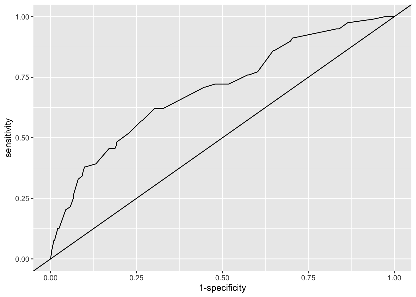
Figure 6.7: ROC curve for our logistic regression model of the indo RCT data (solid line). The line y=x shows the ROC curve we’d expect with random guessing.
and find the area under the curve for the model
## Area under the curve: 0.7So we see that our model is better than random guessing, but really not all that good! In particular, wherever we put a threshold (if we use the model that way), many people will be mis-classified. It’s also worth noting that here we’re performing the diagnostics on the data we used to fit the model: if we were to use the model on a new set of patients, the fit would likely be slightly worse.
6.4.2 Calibration
In this section we are thinking of the model as actually predicting probabilities, and therefore we want to determine whether these probabilities are, in some sense, ‘correct’ or ‘accurate’. One intuitive way to do this is to work through different ‘types’ of patient (by which we mean different combinations of baseline covariate values) and see whether the proportions of ones in the data broadly match the probability given by the model.
If the explanatory variables are factors, and we have repeated observations for the different combinations of factor levels, then for each combination we can estimate the probability of success (or whatever our outcome variable is) using the data, and compare this to the fitted model value.
Example 6.13 This example uses the model fitted in Example 6.10.
The trial has 602 participants and there are many fewer than 602 combinations of the above factor variables, so for many such combinations we will have estimates. Since we are in three dimensions, plotting the data is moderately problematic. We will have a plot for each site (or for the two main ones), use risk score for the \(x\) axis and colour points by treatment group. The circles show the proportions of ones in the data, and are sized by the number of observations used to calculate that estimate. The dashed lines and ribbons show the mean and 95% CI of the fitted value.
## what columns do I want?
# site, risk, rx
# minus one for mean because outcome is 1 or 2
indo_sum = indo_rct %>%
  group_by(site, risk, rx) %>%
  summarise(est = mean(as.numeric(outcome))-1, size=length(id), .groups="keep")
indo_sum = indo_sum |>
  filter(site %in% c("1_UM", "2_IU"))

fit_sum = predict(glm_indo, newdata=indo_sum[,1:3], se.fit=T, type="response")

indo_sum$fit = fit_sum$fit
indo_sum$fit_se = fit_sum$se.fit

ggplot(data=indo_sum, aes(x=risk, col=rx)) +
  geom_point(aes(y=est, size=size), pch=16) +
  geom_line(aes(x=risk, y=fit, col=rx), linetype=2) +
  geom_ribbon(
    aes(
      x=risk,
      ymin=fit-1.96*fit_se,
      ymax=fit+1.96*fit_se,
      fill = rx
      ),
    alpha =0.3)+
  theme_bw()+
  facet_wrap("site") + theme(legend.position = "bottom")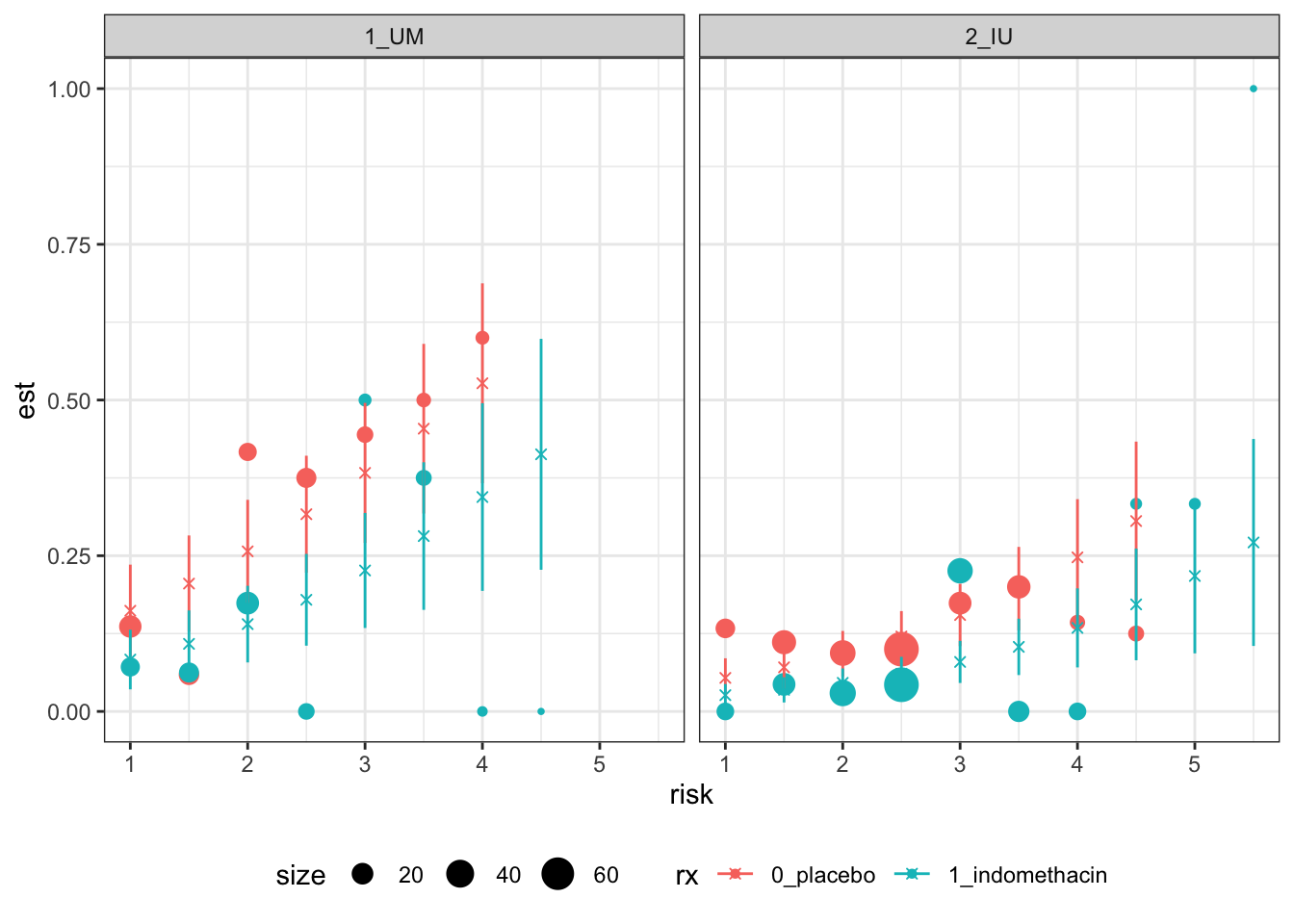
Figure 6.8: Calibration-based plots for indo RCT data for sites 1 (left) and 2 (right).
These plots are not the easiest to interpret, but there seems to be no evidence of systematic trends away from the model.
We will look some more at this in the upcoming practical class, as well as some further principles of model validation.
For now, we’re done with Binary data, and in our next few lectures we’ll think about survival, or time-to-event data.